Demographic Modeling - Cluster analysis
In this topic, we will discuss Unsupervised Learning, or as we talked about last time, the situation where you are looking for groups in your data when your data don’t come with a group variable. I.e. sometimes you want to find groups of similar observations, and you need a statistical tool for doing this.
In statistics, this is called Cluster analysis, another case of the machine learning people inventing a new word for something and taking credit for a type of analysis that’s been around for fifty years.
Cluster analysis
- Attempts to find sub-groups within a data set
- Observations within a particular sub-gruop are statistically more similar to other members of their sub-group than to members of another sub-group
- Many ways in which to do this:
- K-means/K-medioids
- Hierarchical clustering
- Model based clustering
- Latent class analysis
- All of these methods use observed data to measure the dissimilarity between observations, then create groups, or clusters (buckets) from these observations.
Metrics of similiarity
- Distance based
- Euclidean distances between two observations, i and j is
\[d(x_i,x_j) = \sqrt{(x_i-x_j)'(x_i-x_j)}\]
Where the x’s are the variables measured on the two observations, for instance, if we have 3 x variables for two observations, then the distance between them is:
##          x1
## x2 5.744563
If the two observations are more similar, the distance is smaller:
##           x1        x2
## x2  3.162278
## x3 11.575837 11.747340
and vice versa.
library(readr)
prb<-read_csv(file = "https://raw.githubusercontent.com/coreysparks/data/master/PRB2008_All.csv", col_types = read_rds(url("https://raw.githubusercontent.com/coreysparks/r_courses/master/prbspec.rds")))
names(prb)<-tolower(names(prb))

library(dplyr)
##
## Attaching package: 'dplyr'## The following objects are masked from 'package:stats':
##
## filter, lag## The following objects are masked from 'package:base':
##
## intersect, setdiff, setequal, unionprb<-prb%>%
# mutate(africa=ifelse(continent=="Africa", 1, 0))%>%
filter(complete.cases(imr, tfr, percpoplt15, e0total, percurban, percmarwomcontramodern))%>%
select(imr, tfr, percpoplt15, e0total, percurban, percmarwomcontramodern)| imr | tfr | percpoplt15 | e0total | percurban | percmarwomcontramodern |
|---|---|---|---|---|---|
| 163.0 | 6.8 | 45 | 43 | 20 | 9 |
| 8.0 | 1.6 | 27 | 75 | 45 | 8 |
| 27.0 | 2.3 | 30 | 72 | 63 | 52 |
| 132.0 | 6.8 | 46 | 43 | 57 | 5 |
| 26.0 | 1.7 | 21 | 71 | 64 | 20 |
| 4.7 | 1.9 | 19 | 81 | 87 | 75 |
Create data partition
Here we use 80% of the data to train our simple model
## Loading required package: lattice## Loading required package: ggplot2## Warning: The `i` argument of ``[`()` can't be a matrix as of tibble 3.0.0.
## Convert to a vector.
## This warning is displayed once every 8 hours.
## Call `lifecycle::last_warnings()` to see where this warning was generated.Hierarchical clustering
First we form our matrix of distances between all the countries on our observed variables:
Then we run a hierarhical clustering algorithm on the matrix. There are lots of different ways to do this, we will just use the simplest method, the single-linkage, or nearest neighbor approach. This works by first sorting the distances from smallest to largest, then making clusters from the smallest distance pair.
Once this is done, this pair is merged into a cluster, their distance is then compared to the remaining observations, so on and so on, until you have a set of clusters for every observation.
The original way to plot these analyses is by a dendrogram, or tree plot.
hc1<-hclust(d= dmat, method="single")
plot(hc1, hang=-1, main="Single linkage cluster analysis of PRB data")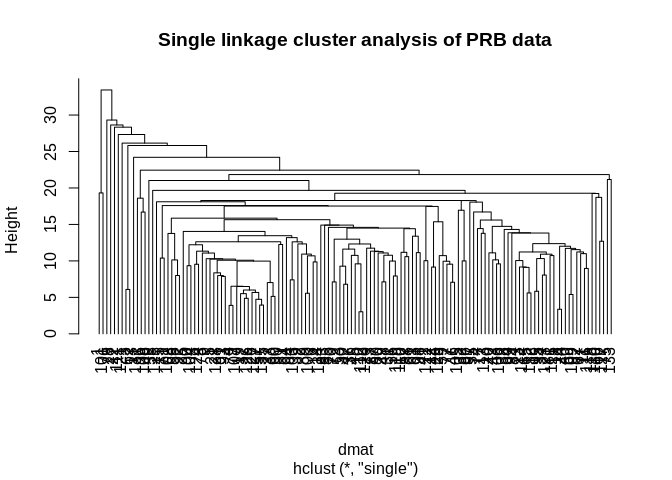
## Welcome! Want to learn more? See two factoextra-related books at https://goo.gl/ve3WBalibrary(class)
library(RColorBrewer)
fviz_dend(hc1, k=5, k_colors =brewer.pal(n=5, name="Accent"),
color_labels_by_k = TRUE, ggtheme = theme_minimal())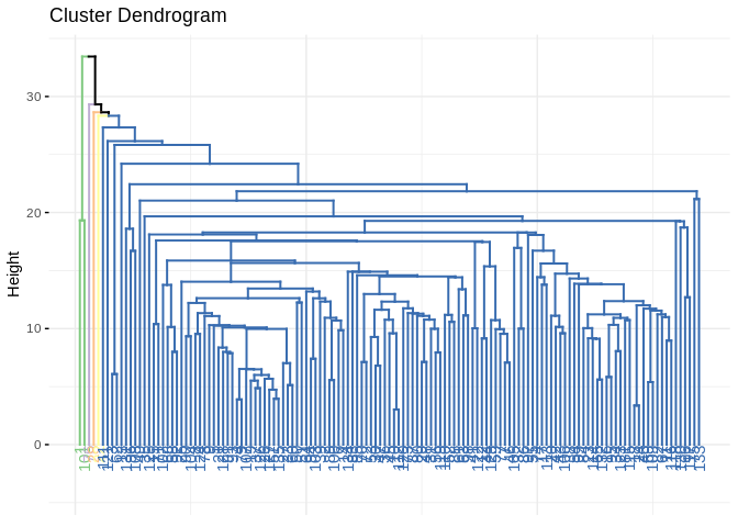
## groups
##   1   2   3   4   5
##   2 130   1   1   1
So this is silly becuase the method round 3 cluster that only had one observation. This is a weakness of the single linkage method, instead we use another method. Ward’s method is typically seen as a better alternative because it tends to find clusters of similar size.
hc2<-hclust(d= dmat, method="ward.D")
plot(hc2, hang=-1, main="Ward's cluster analysis of PRB data")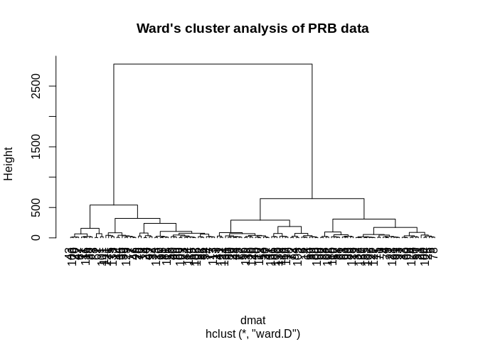
fviz_dend(hc2, k=5, k_colors = brewer.pal(n=5, name="Accent"),
          color_labels_by_k = TRUE, ggtheme = theme_minimal())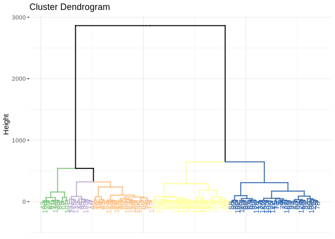
## groups
##  1  2  3  4  5
## 13 38 43 12 29prbtrain$group1<-factor(cutree(hc2, k=5))
prbtrain%>%
ggplot(aes(x=imr, y=tfr, pch=group1,color=group1, cex=3))+geom_point()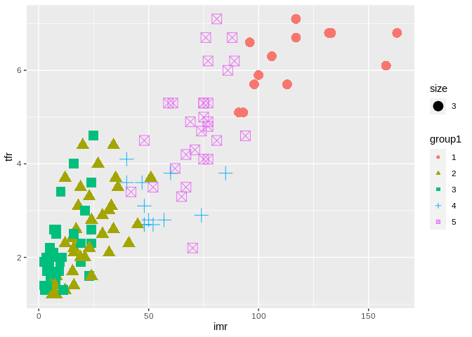
K-means
- Another type of cluster finder
- Will always find a given number of k clusters.
- Ideally we can minimize a within cluster variance measure to find the optimal number
## K-means clustering with 3 clusters of sizes 41, 56, 38
##
## Cluster means:
##        imr      tfr percpoplt15  e0total percurban percmarwomcontramodern
## 1 88.31707 5.263415    42.70732 54.39024  35.39024               15.12195
## 2 11.75536 2.035714    22.50000 75.23214  75.03571               53.71429
## 3 31.74737 2.915789    32.34211 66.92105  38.28947               41.86842
##
## Clustering vector:
##   [1] 1 3 1 2 2 3 3 2 2 3 1 3 3 3 2 1 1 1 2 1 2 2 1 1 2 2 2 1 2 3 2 1 2 1 3 3 2
##  [38] 1 3 1 3 1 1 3 3 3 3 2 1 2 2 2 3 1 3 2 2 2 3 2 2 1 2 2 1 3 1 2 1 3 2 3 3 1
##  [75] 3 2 3 2 2 2 1 1 2 1 2 1 3 2 2 2 2 2 2 2 1 3 1 2 1 2 1 2 2 2 3 1 2 3 1 2 1
## [112] 3 1 1 1 1 3 3 2 2 1 3 1 2 2 2 2 2 3 3 3 1 3 3 2
##
## Within cluster sum of squares by cluster:
## [1] 44040.58 38082.11 30145.52
##  (between_SS / total_SS =  68.8 %)
##
## Available components:
##
## [1] "cluster"      "centers"      "totss"        "withinss"     "tot.withinss"
## [6] "betweenss" "size" "iter" "ifault"## Loading required package: gtoolskm2<-KMeans_rcpp(data=prbtrain, cluster=3, num_init = 10)
prbtrain$cluster<-as.factor(km2$cluster)
prbtrain%>%
ggplot(aes(x=imr, y=tfr, group=cluster, color=cluster, cex=3))+geom_point()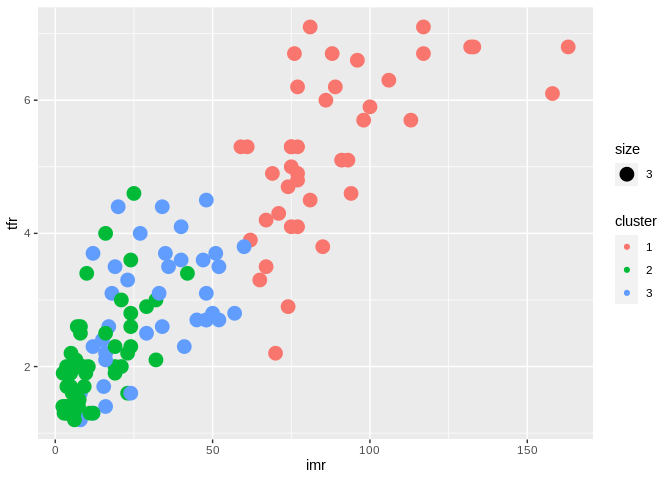
Finding optimal number of clusters
Here I loop over 1 to 10 clusters and store the between group variances, then plot the relative differences. You are looking for the number of clusters where you see a shoulder in the plot.
ss<-NULL
for(i in 1:10){
  km<-kmeans(x=prbtrain, nstart = 10, centers = i)
  ss[i]<-km$betweenss / km$totss

}

plot(x=2:10, y=diff(ss))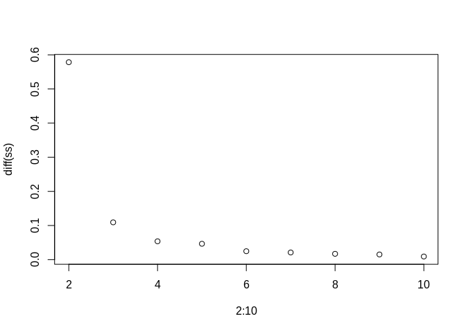
Looks like the difference in variances stops declining dramatically at k=3 clusters.
Here are the test cases plotted as X’s
prbtest$cluster<-as.factor(predict_KMeans(data=prbtest, CENTROIDS = km2$centroids))

prbtest%>%
  ggplot(aes(x=imr, y=tfr, group=cluster, color=cluster,cex=1.5))+geom_point(aes(cex=2.5) ,pch="x")+geom_point(data=prbtrain, aes(x=imr, y=tfr, group=cluster, color=cluster))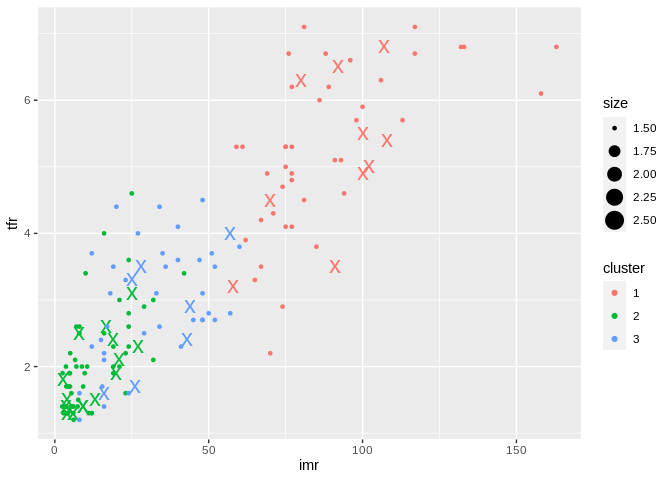
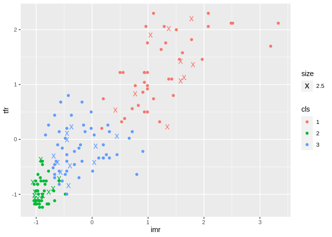
Gaussian mixtures
- These are a type of clustering method that is based on finding a finite mixture of Gaussian distributions within data.
- Only useful for continuous variables in data
prbtrain<-prb[train,]
prbtest<-prb[-train,]

prbtrain<-center_scale(prb[train,])
prbtest<-center_scale(prb[-train,])

plot(Optimal_Clusters_GMM(data = prbtrain, max_clusters = 10,seed_mode = "random_subset", km_iter = 20, em_iter = 20))

gmprb<-GMM(data = prbtrain, gaussian_comps = 3,seed_mode = "random_subset", km_iter = 10, em_iter = 10)

#gmprbprbtrain<-data.frame(prbtrain)
names(prbtrain)<-names(prb)
prbtrain$cls<-as.factor(apply(gmprb$Log_likelihood, 1, which.max))
pred<-predict_GMM(data=prbtest, CENTROIDS = gmprb$centroids, COVARIANCE = gmprb$covariance_matrices, WEIGHTS = gmprb$weights)
prbtest<-data.frame(prbtest)
names(prbtest)<-names(prb)
prbtest$cls<-as.factor(pred$cluster_labels+1)
prbtest%>%
ggplot(aes(x=imr, y=tfr, group=cls, color=cls))+geom_point(pch="x", aes(cex=2.5) )+geom_point(data=prbtrain, aes(x=imr, y=tfr, group=cls, color=cls))