Demography Informal Methods Seminar - Lasso and Regularized Regression
Regularization in Regression
I would suggest you read Chapter 6 and especially section 6.2 of An Introduction to Statistical Learning to get a full treatment of this topic.
If you want to read the sources for the Lasso, check out the paper by Friedman, Hastie and Tibshirani (2010)
Why do I want to talk about this? The Lasso and regularization are a popular technique in data science today that allows you to perform both variable selection and optimized prediction in one algorithm. It also can alleviate some problems of multicollinearity between predictors. The Lasso can be applied to linear, generalized linear, generalized linear mixed models and the Cox model, and there are R packages that provide this functionality.
We will first have a look at the linear model solution and extend it.
The good ol’ (generalized) linear model
Linear regression
The standard linear regression can be written:
\[\hat y = \hat \beta_0 + \sum {\hat \beta_k x_{ik}}\]
where the terms on the right correspond to the linear predictor for the outcome (\(y\)), given the values of the predictors (\(x_k\)). The \(\hat \beta\) values are the unbiased estimates of the regression parameters, for the linear model, typically found by least squares estimation.
Generalized linear model
Extension of the linear modeling concept to non-gaussian outcomes.
Link function \(\eta\) links the mean of the outcome to a linear predictor with a nonlinear function \(\eta\)
E.G. Logistic regression -
\[log \left( \frac{p_i}{1-p_i} \right ) =\eta_i = \sum {\beta_k x_{ik}}\] To get the probability from the model, we use the inverse logit transform: \[p_i = \frac{1}{1+exp^{\eta}}\]
Model estimation
Find the parameters of the model so that the model Deviance is minimized. In the linear regression context, Deviance is the same as the Residual Squared Error or Residual Sums of Squares
\[\text{Deviance} = \sum (y_i - \sum{\hat{\beta_k x_{ik}}}) ^2 \]
The problem is when there are parameters in the model that are zero or nearly zero, the model may have higher deviance than it could if some of those parameters were not in the model.
The question is how to go about doing this?
You may have seen methods of regression subsetting via stepwise, forward or backward selection. These methods iteratively insert or remove predictor variables from the model, and in this process the models are scored via either their RSS or AIC or some other information criteria.
Here is an example where we fit a linear model and the perform variable subset selection.
##
## Attaching package: 'dplyr'
## The following objects are masked from 'package:stats':
##
## filter, lag## The following objects are masked from 'package:base':
##
## intersect, setdiff, setequal, union## Warning: Number of logged events: 655A common data science approach would be to fit a model with all predictors included, and then winnow the model to include only the significant predictors. We start with this type of model:
##
## Attaching package: 'MASS'
## The following object is masked from 'package:dplyr':
##
## selectX<-scale(model.matrix(e0total~. , data=prb2))
dat<-data.frame(X[,-1])
dat$y<-prb2$e0total
fm<-glm(y~., data=dat)
summary(fm)##
## Call:
## glm(formula = y ~ ., data = dat)
##
## Deviance Residuals:
## Min 1Q Median 3Q Max
## -4.3470 -1.0362 0.1334 0.9305 8.1069
##
## Coefficients:
## Estimate Std. Error t value Pr(>|t|)
## (Intercept) 67.95694 0.12294 552.744 < 2e-16 ***
## continentAsia 0.07720 0.20327 0.380 0.7045
## continentEurope 0.22202 0.29448 0.754 0.4519
## continentNorth.America 0.39021 0.19561 1.995 0.0475 *
## continentOceania -0.10322 0.17471 -0.591 0.5554
## continentSouth.America 0.24651 0.16210 1.521 0.1301
## population. -0.07920 0.13370 -0.592 0.5543
## cbr -6.23299 3.19702 -1.950 0.0527 .
## cdr -2.37212 1.31148 -1.809 0.0721 .
## rate.of.natural.increase 5.53259 2.88553 1.917 0.0568 .
## net.migration.rate -0.11659 0.20356 -0.573 0.5675
## imr -2.37542 0.42992 -5.525 1.12e-07 ***
## womandlifetimeriskmaternaldeath 0.06185 0.21018 0.294 0.7689
## tfr 0.77591 0.87183 0.890 0.3746
## percpoplt15 -0.97796 0.78461 -1.246 0.2142
## percpopgt65 3.02097 0.45506 6.639 3.49e-10 ***
## percurban -0.10826 0.23176 -0.467 0.6410
## percpopinurbangt750k 0.30498 0.21709 1.405 0.1618
## percpop1549hivaids2007 -1.75795 0.27465 -6.401 1.26e-09 ***
## percmarwomcontraall -0.11868 0.38931 -0.305 0.7608
## percmarwomcontramodern 0.60254 0.33495 1.799 0.0737 .
## percppundernourished0204 -0.28350 0.20518 -1.382 0.1687
## motorvehper1000pop0005 0.37047 0.31006 1.195 0.2337
## percpopwaccessimprovedwatersource 0.33456 0.24727 1.353 0.1777
## gnippppercapitausdollars 0.82764 0.35362 2.341 0.0203 *
## popdenspersqkm 0.30807 0.20080 1.534 0.1267
## ---
## Signif. codes: 0 '***' 0.001 '**' 0.01 '*' 0.05 '.' 0.1 ' ' 1
##
## (Dispersion parameter for gaussian family taken to be 3.159121)
##
## Null deviance: 25164.61 on 208 degrees of freedom
## Residual deviance: 578.12 on 183 degrees of freedom
## AIC: 859.76
##
## Number of Fisher Scoring iterations: 2## [1] 26One traditional approach would then be to do some sort of variable selection, what people used to be taught was stepwise (backward or forward) elmination to obtain the best subset of predictors:
Stepwise selection model
##
## Call:
## glm(formula = y ~ continentNorth.America + continentSouth.America +
##     cbr + cdr + rate.of.natural.increase + imr + percpopgt65 +
##     percpopinurbangt750k + percpop1549hivaids2007 + percmarwomcontramodern +
##     percpopwaccessimprovedwatersource + gnippppercapitausdollars,
##     data = dat)
##
## Deviance Residuals:
##     Min       1Q   Median       3Q      Max
## -4.5939  -1.1511   0.1894   0.9632   8.0198
##
## Coefficients:
##                                   Estimate Std. Error t value Pr(>|t|)
## (Intercept)                        67.9569     0.1213 560.321  < 2e-16 ***
## continentNorth.America              0.3215     0.1300   2.473   0.0142 *
## continentSouth.America              0.2095     0.1317   1.591   0.1132
## cbr                                -6.2002     3.0472  -2.035   0.0432 *
## cdr                                -2.2039     1.2497  -1.764   0.0794 .
## rate.of.natural.increase            5.5896     2.7241   2.052   0.0415 *
## imr                                -2.4789     0.3761  -6.590 3.96e-10 ***
## percpopgt65                         3.6290     0.3294  11.016  < 2e-16 ***
## percpopinurbangt750k                0.2849     0.1498   1.902   0.0586 .
## percpop1549hivaids2007             -1.8568     0.2070  -8.971 2.37e-16 ***
## percmarwomcontramodern              0.3689     0.1699   2.172   0.0311 *
## percpopwaccessimprovedwatersource   0.4307     0.2304   1.870   0.0630 .
## gnippppercapitausdollars            1.2547     0.1883   6.665 2.62e-10 ***
## ---
## Signif. codes:  0 '***' 0.001 '**' 0.01 '*' 0.05 '.' 0.1 ' ' 1
##
## (Dispersion parameter for gaussian family taken to be 3.074258)
##
##     Null deviance: 25164.61  on 208  degrees of freedom
## Residual deviance:   602.55  on 196  degrees of freedom
## AIC: 842.41
##
## Number of Fisher Scoring iterations: 2## [1] 13Sure enough, there are fewer predictors in the model, and those that remain have small p values.
We can also see the relative model fits of the two models:
## [1] 859.7625## [1] 842.4147This shows that the original model had 26 parameters, while the model that used AIC to find the best subset had 13 parameters, and the relative model fit, in terms of AIC went from 859.762467 for the saturated model to 842.4147049 for the stepwise model.
An alternative to stepwise selection is called Best Subset Regression and considers all possible combinations of variables from the data, and scores the model based on seeing all possible predictors.
## Loading required package: leapsyx<-data.frame(cbind(X[,-1],prb2$e0total))
b1<-bestglm(yx,IC = "AIC", family=gaussian, method = "exhaustive")
summary(b1$BestModel)##
## Call:
## lm(formula = y ~ ., data = data.frame(Xy[, c(bestset[-1], FALSE),
## drop = FALSE], y = y))
##
## Residuals:
## Min 1Q Median 3Q Max
## -4.5939 -1.1511 0.1894 0.9632 8.0198
##
## Coefficients:
## Estimate Std. Error t value Pr(>|t|)
## (Intercept) 67.9569 0.1213 560.321 < 2e-16 ***
## continentNorth.America 0.3215 0.1300 2.473 0.0142 *
## continentSouth.America 0.2095 0.1317 1.591 0.1132
## cbr -6.2002 3.0472 -2.035 0.0432 *
## cdr -2.2039 1.2497 -1.764 0.0794 .
## rate.of.natural.increase 5.5896 2.7241 2.052 0.0415 *
## imr -2.4789 0.3761 -6.590 3.96e-10 ***
## percpopgt65 3.6290 0.3294 11.016 < 2e-16 ***
## percpopinurbangt750k 0.2849 0.1498 1.902 0.0586 .
## percpop1549hivaids2007 -1.8568 0.2070 -8.971 2.37e-16 ***
## percmarwomcontramodern 0.3689 0.1699 2.172 0.0311 *
## percpopwaccessimprovedwatersource 0.4307 0.2304 1.870 0.0630 .
## gnippppercapitausdollars 1.2547 0.1883 6.665 2.62e-10 ***
## ---
## Signif. codes: 0 '***' 0.001 '**' 0.01 '*' 0.05 '.' 0.1 ' ' 1
##
## Residual standard error: 1.753 on 196 degrees of freedom
## Multiple R-squared: 0.9761, Adjusted R-squared: 0.9746
## F-statistic: 665.8 on 12 and 196 DF, p-value: < 2.2e-16This creates a parsimonious model, with only 13 coefficients and an AIC of 842.4147049 which is slightly lower than the stepwise model.
Model shrinkage
Variable selection methods are one way to approach finding the most parsimonious model in an analysis, but alternative methods also exist. The modern approach to doing this is lumped under the term shrinkage methods

As opposed to the variable selection methods, shrinkage models fit a model that contains all the predictors in the data, and constrains or regularizes the coefficients so that they shrink towards 0, effectively eliminating the unnecessary parameters from the model.
There are two main classes of these methods, Ridge regression and the Lasso.
Ridge regression
Ridge regression is very similar to other regression methods, except the estimates are estimated using a slightly different objective criteria. The estimates of the model coefficient are estimates so that the quantity:
\[\text{Penalized Deviance} = \sum (y_i - \sum{\hat{\beta_k x_k}}) ^2 + \lambda \sum_k \beta_k^2 = \text{Deviance} + \lambda \sum_k \beta_k^2\] is minimized. This looks a lot like the ordinary Deviance for the models above, except it adds a penalization term to the fit criteria. The term \(\lambda\), \(\lambda \geq 0\) is a tuning parameter. The Ridge regression coefficients are those that both fit the data well, and penalize the deviance the least.
Then penalty term is small when the \(\beta\)s are close to 0. As the value of \(\lambda\) increases, the coefficients will be forced to 0. This implies another set of estimation so that the “best” value for \(\lambda\) can be found.
Unlike regular regression, which produces 1 set of regression parameters, the Ridge regression produces a set of regression parameters, each one for a given value of \(\lambda\). The best value for \(\lambda\) is found by a grid search over a range of values.
Here is an example
## Loading required package: Matrix## Loaded glmnet 4.0-2x<-X[,-1]
y<-as.matrix(yx[, 26])
ridgemod<-glmnet(x=x,y=y, alpha = 0, nlambda = 100)
plot(ridgemod, label = T, xvar = "lambda")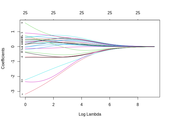
So, the y axis represents the value of the \(\beta\)’s from the model, and the x axis are the various values of \(\lambda\) for each specific value of \(\lambda\). As you see when \(\lambda\) is 0, the coefficients can be quite large, and as \(\lambda\) increase, the \(\beta\)’s converge to 0. This is nice, but we need to find a “best” value of \(\lambda\). This is done via cross-validation, typically.
##
## Call:  cv.glmnet(x = x, y = y, family = "gaussian", alpha = 0)
##
## Measure: Mean-Squared Error
##
##     Lambda Measure     SE Nonzero
## min 0.9822   4.382 0.5652      25
## 1se 2.2690   4.908 0.4604      25
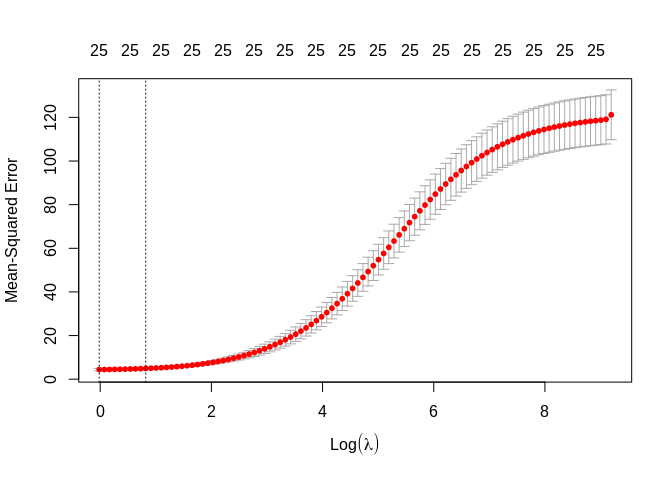
The plot shows the mean square error for the model with a particular value of log(\(\lambda\)). The dotted lines represent the “best” value and the value of \(\lambda\) that is 1 standard error larger than the true minimum.
Why the two values? Well, the minimum value of \(\lambda\), in this case about -0.0179864, and the minimum + 1se is 0.8193173. The smaller value gives the simplest model, while the 1 se value gives the simplest model that also has high accuracy.
How do the coefficient compare?
##
## Call:  glmnet(x = x, y = y, alpha = 0, lambda = s1$lambda.min)
##
##   Df  %Dev Lambda
## 1 25 97.32 0.9822## 25 x 1 sparse Matrix of class "dgCMatrix"
## s0
## continentAsia 0.16976947
## continentEurope 0.34553181
## continentNorth America 0.46350047
## continentOceania -0.02282180
## continentSouth America 0.27165406
## population. -0.10805054
## cbr -0.77128773
## cdr -3.19773064
## rate.of.natural.increase 0.74050874
## net.migration.rate -0.19158308
## imr -2.21869216
## womandlifetimeriskmaternaldeath 0.27651883
## tfr -0.35993995
## percpoplt15 -0.65751353
## percpopgt65 1.59794019
## percurban -0.02204929
## percpopinurbangt750k 0.36644454
## percpop1549hivaids2007 -2.34569547
## percmarwomcontraall 0.15264335
## percmarwomcontramodern 0.57816390
## percppundernourished0204 -0.34197021
## motorvehper1000pop0005 0.66058433
## percpopwaccessimprovedwatersource 0.58660140
## gnippppercapitausdollars 0.91519991
## popdenspersqkm 0.46516889df1<-data.frame(names = names(coef(fm)) , beta=round(coef(fm),4), mod="gm")
df2<-data.frame(names = c(names(coef(fm)[1]), row.names(ridgemod2$beta)), beta=round(as.numeric(coef(s1, s = s1$lambda.min)),4), mod="ridge")
dfa<-rbind(df1, df2)
library(ggplot2)
dfa%>%
ggplot()+geom_point(aes(y=beta,x=names, color=mod))+theme_minimal()+theme(axis.text.x = element_text(angle = 45, vjust = 0.5, hjust=1))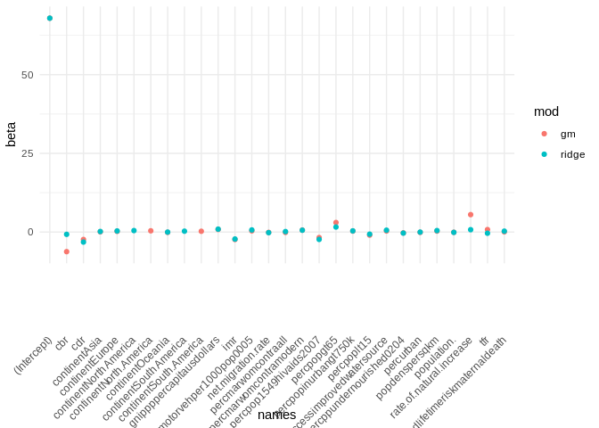
An important note about the ridge regression is that no coefficients are forced to zero, so it is not doing variable selection, only shrinkage of the coefficients. The Lasso, on the other hand can do both.
Lasso

What is the Lasso? Lasso is short for least absolute shrinkage and selection operator. It is designed so that it produces a model that is both strong in the prediction sense, and parsimonious, in that it performs feature (variable) selection as well.
The Lasso is similar to the ridge regression model, in that it penalizes the regression parameter solution, except that the penalty term is not the sum of squared \(\beta\)’s, but the sum of the absolute values of the \(\beta\)’s.
\[ \text{Deviance} + \lambda \sum_k | \beta_k| \]
ridgemod3<-glmnet(x=x,y=y, alpha = 1) #alpha = 1 for Lasso
plot(ridgemod3, label = T, xvar = "lambda")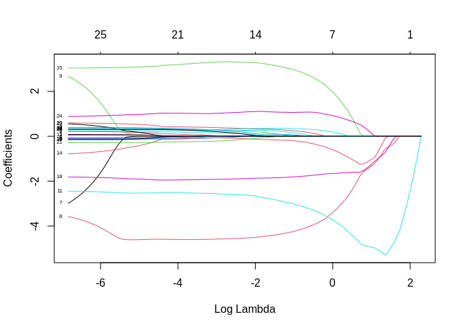
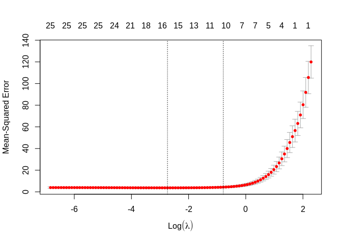
##
## Call:  cv.glmnet(x = x, y = y, family = "gaussian", alpha = 1)
##
## Measure: Mean-Squared Error
##
##     Lambda Measure     SE Nonzero
## min 0.0646   3.731 0.6382      15
## 1se 0.4559 4.352 0.7667 10##
## Call: glmnet(x = x, y = y, family = "gaussian", alpha = 1, lambda = s2$lambda.1se)
##
## Df %Dev Lambda
## 1 10 96.97 0.4559## 25 x 1 sparse Matrix of class "dgCMatrix"
## s0
## continentAsia .
## continentEurope .
## continentNorth America .
## continentOceania .
## continentSouth America .
## population. .
## cbr .
## cdr -4.11173283
## rate.of.natural.increase .
## net.migration.rate .
## imr -3.13251642
## womandlifetimeriskmaternaldeath .
## tfr .
## percpoplt15 -0.25132019
## percpopgt65 2.81422569
## percurban .
## percpopinurbangt750k 0.10711580
## percpop1549hivaids2007 -1.78945838
## percmarwomcontraall .
## percmarwomcontramodern 0.20523750
## percppundernourished0204 .
## motorvehper1000pop0005 0.03841647
## percpopwaccessimprovedwatersource 0.33401182
## gnippppercapitausdollars 1.06967019
## popdenspersqkm .Elastic net
A third method, the Elastic net regression, blends the shrinkage aspects of the ridge regression with the feature selection of the Lasso. This was proposed by Zou and Hastie 2005
\[\text{Deviance} + \lambda [(1-\alpha) \sum_k |\beta_k| + \alpha \sum_k \beta_k^2]\]
ridgemod4<-glmnet(x=x,y=y, alpha = .5, nlambda = 100) #alpha = .5 for elastic net
plot(ridgemod4, label = T, xvar = "lambda")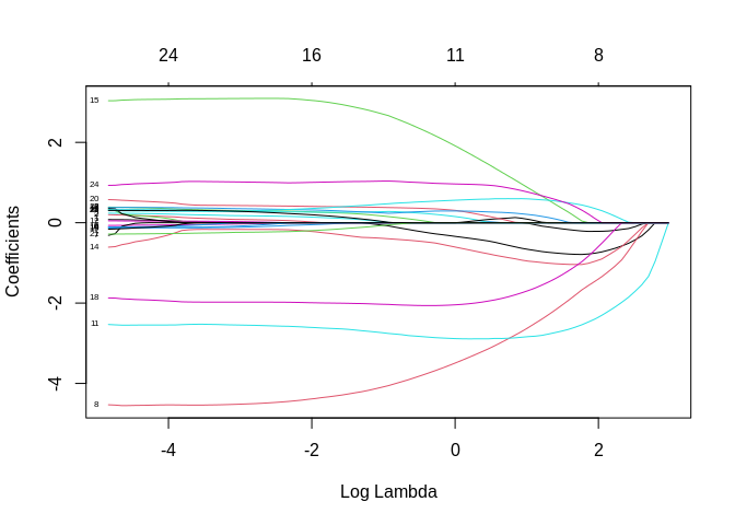
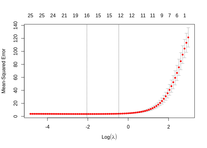
##
## Call:  cv.glmnet(x = x, y = y, family = "gaussian", alpha = 0.5)
##
## Measure: Mean-Squared Error
##
##     Lambda Measure     SE Nonzero
## min 0.1292   3.593 0.5248      16
## 1se 0.6284 4.037 0.5181 12## 25 x 1 sparse Matrix of class "dgCMatrix"
## s0
## continentAsia .
## continentEurope .
## continentNorth America 0.05233114
## continentOceania .
## continentSouth America .
## population. .
## cbr -0.22571539
## cdr -3.79036104
## rate.of.natural.increase .
## net.migration.rate .
## imr -2.84336643
## womandlifetimeriskmaternaldeath .
## tfr .
## percpoplt15 -0.46055079
## percpopgt65 2.31578751
## percurban .
## percpopinurbangt750k 0.23562128
## percpop1549hivaids2007 -2.06460379
## percmarwomcontraall .
## percmarwomcontramodern 0.35690946
## percppundernourished0204 .
## motorvehper1000pop0005 0.28068647
## percpopwaccessimprovedwatersource 0.52328787
## gnippppercapitausdollars 0.99759091
## popdenspersqkm .In these examples, we will use the Demographic and Health Survey Model Data. These are based on the DHS survey, but are publicly available and are used to practice using the DHS data sets, but don’t represent a real country.
In this example, we will use the outcome of contraceptive choice (modern vs other/none) as our outcome. An excellent guide for this type of literature is this article
library(haven)
dat<-url("https://github.com/coreysparks/data/blob/master/ZZIR62FL.DTA?raw=true")
model.dat<-read_dta(dat)
Here we recode some of our variables and limit our data to those women who are not currently pregnant and who are sexually active.
library(dplyr)

model.dat2<-model.dat%>%
  mutate(region = v024,
         modcontra= ifelse(v364 ==1,1, 0),
         age = cut(v012, breaks = 5),
         livchildren=v218,
         educ = v106,
         currpreg=v213,
         wealth = as.factor(v190),
         partnered = ifelse(v701<=1, 0, 1),
         work = ifelse(v731%in%c(0,1), 0, 1),
         knowmodern=ifelse(v301==3, 1, 0),
         age2=v012^2,
         rural = ifelse(v025==2, 1,0),
         wantmore = ifelse(v605%in%c(1,2), 1, 0))%>%
  filter(currpreg==0, v536>0, v701!=9)%>% #notpreg, sex active
dplyr::select(caseid, region, modcontra,age, age2,livchildren, educ, knowmodern, rural, wantmore, partnered,wealth, work)| caseid | region | modcontra | age | age2 | livchildren | educ | knowmodern | rural | wantmore | partnered | wealth | work |
|---|---|---|---|---|---|---|---|---|---|---|---|---|
| 1 1 2 | 2 | 0 | (28.6,35.4] | 900 | 4 | 0 | 1 | 1 | 1 | 0 | 1 | 1 |
| 1 4 2 | 2 | 0 | (35.4,42.2] | 1764 | 2 | 0 | 1 | 1 | 0 | 0 | 3 | 1 |
| 1 4 3 | 2 | 0 | (21.8,28.6] | 625 | 3 | 1 | 1 | 1 | 0 | 0 | 3 | 1 |
| 1 5 1 | 2 | 0 | (21.8,28.6] | 625 | 2 | 2 | 1 | 1 | 1 | 0 | 2 | 1 |
| 1 6 2 | 2 | 0 | (35.4,42.2] | 1369 | 2 | 0 | 1 | 1 | 1 | 0 | 3 | 1 |
| 1 7 2 | 2 | 0 | (15,21.8] | 441 | 1 | 0 | 1 | 1 | 1 | 0 | 1 | 1 |
## Loading required package: latticeset.seed(1115)
train<- createDataPartition(y = model.dat2$modcontra , p = .80, list=F)
dtrain<-model.dat2[train,]## Warning: The `i` argument of ``[`()` can't be a matrix as of tibble 3.0.0.
## Convert to a vector.
## This warning is displayed once every 8 hours.
## Call `lifecycle::last_warnings()` to see where this warning was generated.Logistic regression
library(glmnet)
library(MASS)
fm<-glm(modcontra~region+factor(age)+livchildren+wantmore+rural+factor(educ)+partnered+work+wealth, data = dtrain, family=binomial)
summary(fm)
##
## Call:
## glm(formula = modcontra ~ region + factor(age) + livchildren +
## wantmore + rural + factor(educ) + partnered + work + wealth,
## family = binomial, data = dtrain)
##
## Deviance Residuals:
## Min 1Q Median 3Q Max
## -1.3727 -0.6498 -0.4970 -0.3590 2.5673
##
## Coefficients:
## Estimate Std. Error z value Pr(>|z|)
## (Intercept) -2.80866 0.26506 -10.596 < 0.0000000000000002 ***
## region 0.15475 0.03772 4.103 0.000040825388 ***
## factor(age)(21.8,28.6] 0.44413 0.18439 2.409 0.01601 *
## factor(age)(28.6,35.4] 0.54804 0.19226 2.850 0.00437 **
## factor(age)(35.4,42.2] 0.14667 0.20988 0.699 0.48468
## factor(age)(42.2,49] -0.63063 0.23623 -2.670 0.00760 **
## livchildren 0.18805 0.02976 6.318 0.000000000264 ***
## wantmore -0.16630 0.10204 -1.630 0.10316
## rural -0.62567 0.11323 -5.525 0.000000032859 ***
## factor(educ)1 0.30769 0.13045 2.359 0.01834 *
## factor(educ)2 0.59775 0.13288 4.498 0.000006849378 ***
## factor(educ)3 0.62670 0.24653 2.542 0.01102 *
## partnered 0.28746 0.10467 2.746 0.00603 **
## work 0.16342 0.10386 1.573 0.11561
## wealth2 0.13635 0.14047 0.971 0.33170
## wealth3 0.17350 0.14114 1.229 0.21898
## wealth4 0.24257 0.15013 1.616 0.10614
## wealth5 0.17383 0.18138 0.958 0.33786
## ---
## Signif. codes: 0 '***' 0.001 '**' 0.01 '*' 0.05 '.' 0.1 ' ' 1
##
## (Dispersion parameter for binomial family taken to be 1)
##
## Null deviance: 3818.3 on 4128 degrees of freedom
## Residual deviance: 3536.4 on 4111 degrees of freedom
## AIC: 3572.4
##
## Number of Fisher Scoring iterations: 5stepwise logistic
## Start:  AIC=3572.39
## modcontra ~ region + factor(age) + livchildren + wantmore + rural +
##     factor(educ) + partnered + work + wealth
##
##                Df Deviance    AIC
## - wealth        4   3539.2 3567.2
## <none>              3536.4 3572.4
## - work          1   3538.9 3572.9
## - wantmore      1   3539.0 3573.0
## - partnered     1   3543.8 3577.8
## - region        1   3553.0 3587.0
## - factor(educ)  3   3559.4 3589.4
## - rural         1   3566.7 3600.7
## - livchildren   1   3577.1 3611.1
## - factor(age)   4   3609.4 3637.4
##
## Step:  AIC=3567.21
## modcontra ~ region + factor(age) + livchildren + wantmore + rural +
##     factor(educ) + partnered + work
##
##                Df Deviance    AIC
## <none>              3539.2 3567.2
## - work          1   3541.7 3567.7
## - wantmore      1   3541.8 3567.8
## + wealth        4   3536.4 3572.4
## - partnered     1   3547.9 3573.9
## - region        1   3555.0 3581.0
## - factor(educ)  3   3564.0 3586.0
## - livchildren   1   3579.4 3605.4
## - rural         1   3590.0 3616.0
## - factor(age) 4 3611.8 3631.8## (Intercept) region factor(age)(21.8,28.6]
## -2.6270672 0.1501583 0.4524232
## factor(age)(28.6,35.4] factor(age)(35.4,42.2] factor(age)(42.2,49]
## 0.5612389 0.1621533 -0.6103720
## livchildren wantmore rural
## 0.1861566 -0.1651203 -0.6915328
## factor(educ)1 factor(educ)2 factor(educ)3
## 0.3178917 0.6052986 0.6167321
## partnered work
## 0.3043424 0.1621220Best subset regression
y<-dtrain$modcontra
x<-model.matrix(~factor(region)+factor(age)+livchildren+rural+wantmore+factor(educ)+partnered+work+factor(wealth), data=dtrain)
x<-(x)[,-1]

yx<-as.data.frame(cbind(x[,-1],y))
names(yx)
## [1] "factor(region)3" "factor(region)4" "factor(age)(21.8,28.6]"
## [4] "factor(age)(28.6,35.4]" "factor(age)(35.4,42.2]" "factor(age)(42.2,49]"
## [7] "livchildren" "rural" "wantmore"
## [10] "factor(educ)1" "factor(educ)2" "factor(educ)3"
## [13] "partnered" "work" "factor(wealth)2"
## [16] "factor(wealth)3" "factor(wealth)4" "factor(wealth)5"
## [19] "y"Logistic ridge regression
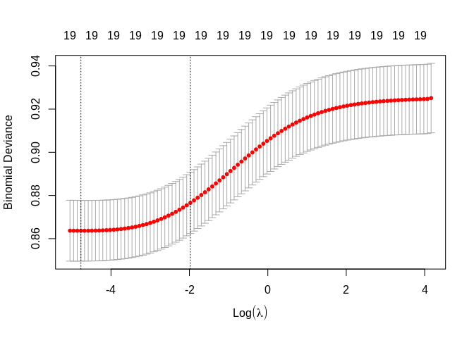
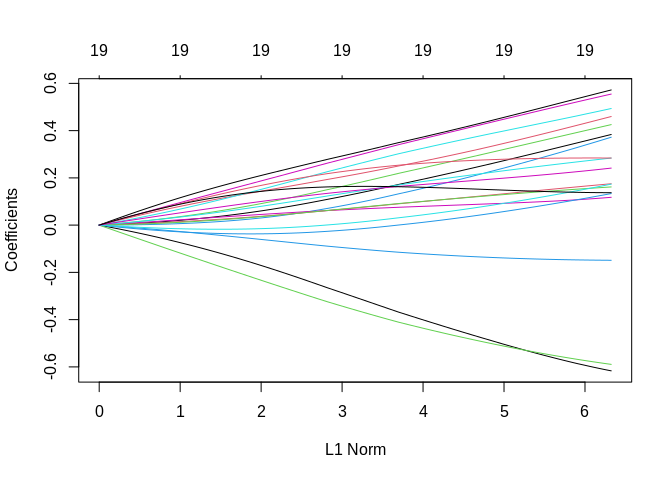
## 19 x 1 sparse Matrix of class "dgCMatrix"
##                                 s0
## factor(region)2         0.11736906
## factor(region)3         0.20097363
## factor(region)4         0.15952400
## factor(age)(21.8,28.6]  0.07831211
## factor(age)(28.6,35.4]  0.23721168
## factor(age)(35.4,42.2]  0.06382724
## factor(age)(42.2,49]   -0.27968879
## livchildren             0.06545045
## rural                  -0.33722253
## wantmore               -0.09296988
## factor(educ)1           0.13004018
## factor(educ)2           0.27349312
## factor(educ)3           0.28825836
## partnered               0.22401406
## work                    0.06631462
## factor(wealth)2        -0.02330795
## factor(wealth)3         0.00422731
## factor(wealth)4         0.13902383
## factor(wealth)5         0.16285245
Logistic Lasso
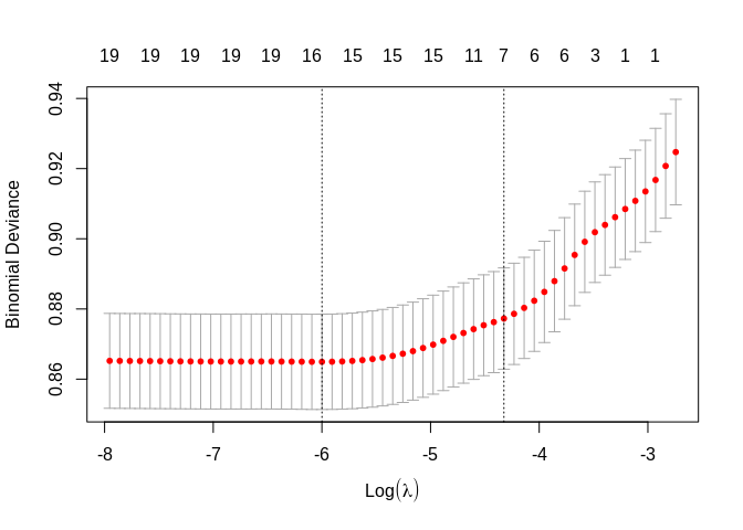
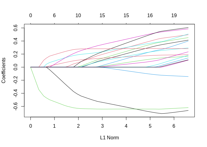
## 19 x 1 sparse Matrix of class "dgCMatrix"
##                                 s0
## factor(region)2         .
## factor(region)3         0.04882613
## factor(region)4         .
## factor(age)(21.8,28.6]  .
## factor(age)(28.6,35.4]  0.17720355
## factor(age)(35.4,42.2]  .
## factor(age)(42.2,49]   -0.37140425
## livchildren             0.09635800
## rural                  -0.62095437
## wantmore                .
## factor(educ)1           .
## factor(educ)2           0.20666302
## factor(educ)3           .
## partnered               0.26927535
## work                    .
## factor(wealth)2         .
## factor(wealth)3         .
## factor(wealth)4         .
## factor(wealth)5         .
classification results
Regular GLM
probabilities <- fm %>% predict(dtest, type = "response")
predicted.classes <- ifelse(probabilities > mean(dtest$modcontra, na.rm=T), 1, 0)
# Prediction accuracy
observed.classes <- dtest$modcontra
mean(predicted.classes == observed.classes, na.rm=T)
## [1] 0.6889535## observed.classes
## predicted.classes 0 1
## 0 605 111
## 1 210 106stepwise logistic model
probabilities <- predict(smod, dtest, type = "response")
predicted.classes <- ifelse(probabilities > mean(dtest$modcontra, na.rm=T), 1, 0)
# Prediction accuracy
observed.classes <- dtest$modcontra
mean(predicted.classes == observed.classes)
## [1] 0.6860465## observed.classes
## predicted.classes 0 1
## 0 605 114
## 1 210 103Logistic ridge regression
x.test <- model.matrix(~factor(region)+factor(age)+livchildren+rural+wantmore+factor(educ)+partnered+work+factor(wealth), data=dtest)
x.test<-(x.test)[,-1]
ytest<-dtrain$modcontra

probabilities <-   predict(object=rmod1, newx = x.test, s=s1$lambda.1se, type="response")
predicted.classes <- ifelse(probabilities > mean(dtest$modcontra), 1,0)
# Model accuracy
observed.classes <- dtest$modcontra
mean(predicted.classes == observed.classes)
## [1] 0.7131783## observed.classes
## predicted.classes 0 1
## 0 646 127
## 1 169 90Logistic Lasso
probabilities <-   predict(object=rmod3, newx = x.test, s=s2$lambda.1se, type="response")
predicted.classes <- ifelse(probabilities > mean(dtest$modcontra), 1,0)
# Model accuracy
observed.classes <- dtest$modcontra
mean(predicted.classes == observed.classes)
## [1] 0.6879845## observed.classes
## predicted.classes 0 1
## 0 611 118
## 1 204 99So what?
By doing any type of regression variable selection, you are going to have the computer tell you what variables are going into your models. A lot of people don’t like this, but it is very common in the applied world in order to build the best models, especially in high-dimensional data.
Take aways
- These methods will lead to more parsimonius models with better predictive power
- The models are sensitive to their tuning parameters, so please don’t jump into this without tuning the model parameters.