Demography Predictive Modeling Working Group - Basic methods for classification
Classification methods and models
In classification methods, we are typically interested in using some observed characteristics of a case to predict a binary categorical outcome. This can be extended to a multi-category outcome, but the largest number of applications involve a 1/0 outcome.
Below, we look at a few classic methods of doing this:
Logistic regression
Regression/Partitioning Trees
Linear Discriminant Functions
There are other methods that we will examine but these are probably the easiest to understand.
In these examples, we will use the Demographic and Health Survey Model Data. These are based on the DHS survey, but are publicly available and are used to practice using the DHS data sets, but don’t represent a real country.
In this example, we will use the outcome of contraceptive choice (modern vs other/none) as our outcome.
library(haven)
dat<-url("https://github.com/coreysparks/data/blob/master/ZZIR62FL.DTA?raw=true")
model.dat<-read_dta(dat)
Here we recode some of our variables and limit our data to those women who are not currently pregnant and who are sexually active.
##
## Attaching package: 'dplyr'
## The following objects are masked from 'package:stats':
##
## filter, lag## The following objects are masked from 'package:base':
##
## intersect, setdiff, setequal, unionmodel.dat2<-model.dat%>%
mutate(region = v024,
modcontra= as.factor(ifelse(v364 ==1,1, 0)),
age = v012,
livchildren=v218,
educ = v106,
currpreg=v213,
knowmodern=ifelse(v301==3, 1, 0),
age2=v012^2)%>%
filter(currpreg==0, v536>0)%>% #notpreg, sex active
dplyr::select(caseid, region, modcontra,age, age2,livchildren, educ, knowmodern)| caseid | region | modcontra | age | age2 | livchildren | educ | knowmodern |
|---|---|---|---|---|---|---|---|
| 1 1 2 | 2 | 0 | 30 | 900 | 4 | 0 | 1 |
| 1 4 2 | 2 | 0 | 42 | 1764 | 2 | 0 | 1 |
| 1 4 3 | 2 | 0 | 25 | 625 | 3 | 1 | 1 |
| 1 5 1 | 2 | 0 | 25 | 625 | 2 | 2 | 1 |
| 1 6 2 | 2 | 0 | 37 | 1369 | 2 | 0 | 1 |
| 1 6 3 | 2 | 0 | 17 | 289 | 0 | 2 | 0 |
using caret to create training and test sets.
We use an 80% training fraction
## Loading required package: lattice## Loading required package: ggplot2set.seed(1115)
train<- createDataPartition(y = model.dat2$modcontra , p = .80, list=F)
model.dat2train<-model.dat2[train,]## Warning: The `i` argument of ``[`()` can't be a matrix as of tibble 3.0.0.
## Convert to a vector.
## This warning is displayed once every 8 hours.
## Call `lifecycle::last_warnings()` to see where this warning was generated.##
## 0 1
## 4036 1409##
## 0 1
## 0.7412305 0.2587695## caseid region modcontra age age2
## Length:5445 Min. :1.000 0:4036 Min. :15.00 Min. : 225.0
## Class :character 1st Qu.:1.000 1:1409 1st Qu.:21.00 1st Qu.: 441.0
## Mode :character Median :2.000 Median :29.00 Median : 841.0
## Mean :2.164 Mean :29.78 Mean : 976.8
## 3rd Qu.:3.000 3rd Qu.:37.00 3rd Qu.:1369.0
## Max. :4.000 Max. :49.00 Max. :2401.0
## livchildren educ knowmodern
## Min. : 0.000 Min. :0.0000 Min. :0.0000
## 1st Qu.: 1.000 1st Qu.:0.0000 1st Qu.:1.0000
## Median : 2.000 Median :0.0000 Median :1.0000
## Mean : 2.546 Mean :0.7381 Mean :0.9442
## 3rd Qu.: 4.000 3rd Qu.:2.0000 3rd Qu.:1.0000
## Max. :10.000 Max. :3.0000 Max. :1.0000Logistic regression for classification
Here we use a basic binomial GLM to estimate the probability of a woman using modern contraception. We use information on their region of residence, age, number of living children and level of education.
This model can be written: \[ln \left ( \frac{Pr(\text{Modern Contraception})}{1-Pr(\text{Modern Contraception})} \right ) = X' \beta\]
Which can be converted to the probability scale via the inverse logit transform:
\[Pr(\text{Modern Contraception}) = \frac{1}{1+exp (-X' \beta)}\]
glm1<-glm(modcontra~factor(region)+scale(age)+scale(age2)+scale(livchildren)+factor(educ), data=model.dat2train[,-1], family = binomial)
summary(glm1)
##
## Call:
## glm(formula = modcontra ~ factor(region) + scale(age) + scale(age2) +
## scale(livchildren) + factor(educ), family = binomial, data = model.dat2train[,
## -1])
##
## Deviance Residuals:
## Min 1Q Median 3Q Max
## -1.4073 -0.7103 -0.5734 1.0669 2.3413
##
## Coefficients:
## Estimate Std. Error z value Pr(>|z|)
## (Intercept) -1.91240 0.06807 -28.095 < 2e-16 ***
## factor(region)2 0.38755 0.08534 4.541 5.60e-06 ***
## factor(region)3 0.62565 0.09531 6.564 5.23e-11 ***
## factor(region)4 0.30066 0.09454 3.180 0.001471 **
## scale(age) 0.63678 0.26540 2.399 0.016425 *
## scale(age2) -0.98328 0.26194 -3.754 0.000174 ***
## scale(livchildren) 0.17004 0.05408 3.144 0.001665 **
## factor(educ)1 0.43835 0.10580 4.143 3.43e-05 ***
## factor(educ)2 1.38923 0.08646 16.068 < 2e-16 ***
## factor(educ)3 1.54061 0.16086 9.577 < 2e-16 ***
## ---
## Signif. codes: 0 '***' 0.001 '**' 0.01 '*' 0.05 '.' 0.1 ' ' 1
##
## (Dispersion parameter for binomial family taken to be 1)
##
## Null deviance: 6226.5 on 5444 degrees of freedom
## Residual deviance: 5629.0 on 5435 degrees of freedom
## AIC: 5649
##
## Number of Fisher Scoring iterations: 4We see that all the predictors are significantly related to our outcome
Next we see how the model performs in terms of accuracy of prediction. This is new comparison to how we typically use logistic regression.
We use the predict() function to get the estimated class probabilities for each case
##          1          2          3          4          5          6
## 0.22002790 0.31137928 0.15091505 0.20389088 0.08726724 0.18808481
These are the estimated probability that each of these women used modern contraception, based on the model.
In order to create classes (uses modern vs doesn’t use modern contraception) we have to use a decision rule. A decision rule is when we choose a cut off point, or threshold value of the probability to classify each observation as belonging to one class or the other.
A basic decision rule is if \(Pr(y=\text{Modern Contraception} |X) >.5\) Then classify the observation as a modern contraception user, and otherwise not. This is what we will use here.
tr_predcl<-factor(ifelse(tr_pred>.5, 1, 0))

library(ggplot2)

pred1<-data.frame(pr=tr_pred, gr=tr_predcl, modcon=model.dat2train$modcontra)

pred1%>%
  ggplot()+geom_density(aes(x=pr, color=gr, group=gr))+ggtitle(label = "Probability of Modern Contraception", subtitle = "Threshold = .5")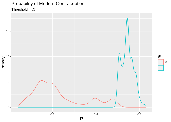
pred1%>%
  ggplot()+geom_density(aes(x=pr, color=modcon, group=modcon))+ggtitle(label = "Probability of Modern Contraception", subtitle = "Truth")
Next we need to see how we did. A simple cross tab of the observed classes versus the predicted classes is called the confusion matrix.
##
## tr_predcl    0    1
##         0 3761 1142
##         1  275  267
This is great, but typically it’s easier to understand the model’s predictive ability by converting these to proportions. The confusionMatrix() function in caret can do this, plus other stuff.
This provides lots of output summarizing the classification results. At its core is the matrix of observed classes versus predicted classes. I got one depiction of this here and from the Wikipedia page
Lots of information on the predictive accuracy can be found from this 2x2 table:
Generally, we are interested in overall accuracy, sensitivity and specificity.
## Confusion Matrix and Statistics
##
##           Reference
## Prediction    0    1
##          0 3761 1142
##          1  275  267
##
##                Accuracy : 0.7398
##                  95% CI : (0.7279, 0.7514)
##     No Information Rate : 0.7412
##     P-Value [Acc > NIR] : 0.6046
##
##                   Kappa : 0.1517
##
##  Mcnemar's Test P-Value : <2e-16
##
##             Sensitivity : 0.9319
##             Specificity : 0.1895
##          Pos Pred Value : 0.7671
##          Neg Pred Value : 0.4926
##              Prevalence : 0.7412
##          Detection Rate : 0.6907
##    Detection Prevalence : 0.9005
##       Balanced Accuracy : 0.5607
##
##        'Positive' Class : 0
##
Overall the model has a 73.9% accuracy, which isn’t bad! What is bad is some of the other measures. The sensitivity is really low 267/(267+1142) = .189, so we are only predicting the positive class (modern contraception) in 19% of cases correctly. In other word the model is pretty good at predicting if you don’t use modern contraception, 3761/(3761+275)= .931, but not at predicting if you do.
We could try a different decision rule, in this case, I use the mean of the response as the cutoff value.
tr_predcl<-factor(ifelse(tr_pred>.258, 1, 0)) #mean of response

pred2<-data.frame(pr=tr_pred, gr=tr_predcl, modcon=model.dat2train$modcontra)
pred2%>%
  ggplot()+geom_density(aes(x=pr, color=gr, group=gr))+ggtitle(label = "Probability of Modern Contraception", subtitle = "Threshold = .258")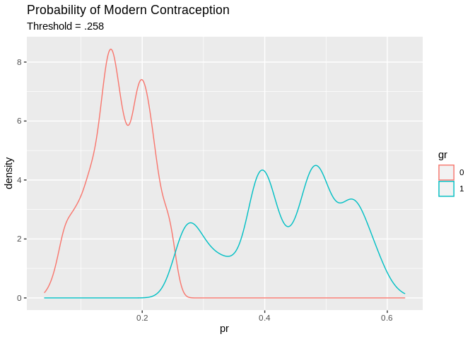
pred2%>%
  ggplot()+geom_density(aes(x=pr, color=modcon, group=modcon))+ggtitle(label = "Probability of Modern Contraception", subtitle = "Truth")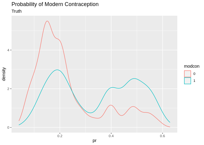
## Confusion Matrix and Statistics
##
##           Reference
## Prediction    0    1
##          0 2944  577
##          1 1092  832
##
##                Accuracy : 0.6935
##                  95% CI : (0.681, 0.7057)
##     No Information Rate : 0.7412
##     P-Value [Acc > NIR] : 1
##
##                   Kappa : 0.2859
##
##  Mcnemar's Test P-Value : <2e-16
##
##             Sensitivity : 0.5905
##             Specificity : 0.7294
##          Pos Pred Value : 0.4324
##          Neg Pred Value : 0.8361
##              Prevalence : 0.2588
##          Detection Rate : 0.1528
##    Detection Prevalence : 0.3534
##       Balanced Accuracy : 0.6600
##
##        'Positive' Class : 1
##
Which drops the accuracy a little, but increases the specificity at the cost of the sensitivity.
Next we do this on the test set to evaluate model performance outside of the training data
pred_test<-predict(glm1, newdata=model.dat2test, type="response")
pred_cl<-factor(ifelse(pred_test>.28, 1, 0))

table(model.dat2test$modcontra,pred_cl)
## pred_cl
## 0 1
## 0 746 262
## 1 160 192## Confusion Matrix and Statistics
##
## Reference
## Prediction 0 1
## 0 746 160
## 1 262 192
##
## Accuracy : 0.6897
## 95% CI : (0.6644, 0.7142)
## No Information Rate : 0.7412
## P-Value [Acc > NIR] : 1
##
## Kappa : 0.2609
##
## Mcnemar's Test P-Value : 8.806e-07
##
## Sensitivity : 0.7401
## Specificity : 0.5455
## Pos Pred Value : 0.8234
## Neg Pred Value : 0.4229
## Prevalence : 0.7412
## Detection Rate : 0.5485
## Detection Prevalence : 0.6662
## Balanced Accuracy : 0.6428
##
## 'Positive' Class : 0
## Regression partition tree
As we saw in the first working group example, the regression tree is another common technique used in classification problems. Regression or classification trees attempt to
library(rpart)
library(rpart.plot)

rp1<-rpart(modcontra~factor(region)+(age)+livchildren+factor(educ),
           data=model.dat2train,
           method ="class",
           control = rpart.control(minbucket = 10, cp=.01)) #lower CP parameter makes for more compliacted tree
summary(rp1)
## Call:
## rpart(formula = modcontra ~ factor(region) + (age) + livchildren +
## factor(educ), data = model.dat2train, method = "class", control = rpart.control(minbucket = 10,
## cp = 0.01))
## n= 5445
##
## CP nsplit rel error xerror xstd
## 1 0.04009936 0 1.0000000 1.0000000 0.02293618
## 2 0.01100071 2 0.9198013 0.9198013 0.02230305
## 3 0.01000000 4 0.8977999 0.9169624 0.02227934
##
## Variable importance
## factor(educ) livchildren age factor(region)
## 58 23 19 1
##
## Node number 1: 5445 observations, complexity param=0.04009936
## predicted class=0 expected loss=0.2587695 P(node) =1
## class counts: 4036 1409
## probabilities: 0.741 0.259
## left son=2 (3862 obs) right son=3 (1583 obs)
## Primary splits:
## factor(educ) splits as LLRR, improve=189.73590, (0 missing)
## livchildren < 0.5 to the right, improve= 84.51811, (0 missing)
## age < 23.5 to the right, improve= 52.42664, (0 missing)
## factor(region) splits as LLRL, improve= 36.53020, (0 missing)
## Surrogate splits:
## livchildren < 0.5 to the right, agree=0.772, adj=0.215, (0 split)
## age < 19.5 to the right, agree=0.753, adj=0.149, (0 split)
## factor(region) splits as LLRL, agree=0.713, adj=0.014, (0 split)
##
## Node number 2: 3862 observations
## predicted class=0 expected loss=0.174262 P(node) =0.7092746
## class counts: 3189 673
## probabilities: 0.826 0.174
##
## Node number 3: 1583 observations, complexity param=0.04009936
## predicted class=0 expected loss=0.46494 P(node) =0.2907254
## class counts: 847 736
## probabilities: 0.535 0.465
## left son=6 (868 obs) right son=7 (715 obs)
## Primary splits:
## livchildren < 0.5 to the right, improve=33.940940, (0 missing)
## age < 36.5 to the right, improve=20.441730, (0 missing)
## factor(region) splits as LRRL, improve= 2.382434, (0 missing)
## factor(educ) splits as --LR, improve= 0.556353, (0 missing)
## Surrogate splits:
## age < 20.5 to the right, agree=0.749, adj=0.443, (0 split)
##
## Node number 6: 868 observations
## predicted class=0 expected loss=0.3709677 P(node) =0.1594123
## class counts: 546 322
## probabilities: 0.629 0.371
##
## Node number 7: 715 observations, complexity param=0.01100071
## predicted class=1 expected loss=0.420979 P(node) =0.1313131
## class counts: 301 414
## probabilities: 0.421 0.579
## left son=14 (14 obs) right son=15 (701 obs)
## Primary splits:
## age < 32.5 to the right, improve=9.574909, (0 missing)
## factor(educ) splits as --LR, improve=1.650766, (0 missing)
## factor(region) splits as LRRL, improve=1.324512, (0 missing)
##
## Node number 14: 14 observations
## predicted class=0 expected loss=0 P(node) =0.002571166
## class counts: 14 0
## probabilities: 1.000 0.000
##
## Node number 15: 701 observations, complexity param=0.01100071
## predicted class=1 expected loss=0.4094151 P(node) =0.128742
## class counts: 287 414
## probabilities: 0.409 0.591
## left son=30 (137 obs) right son=31 (564 obs)
## Primary splits:
## age < 16.5 to the left, improve=7.933444, (0 missing)
## factor(educ) splits as --LR, improve=2.545437, (0 missing)
## factor(region) splits as LRRL, improve=1.768127, (0 missing)
##
## Node number 30: 137 observations
## predicted class=0 expected loss=0.4379562 P(node) =0.0251607
## class counts: 77 60
## probabilities: 0.562 0.438
##
## Node number 31: 564 observations
## predicted class=1 expected loss=0.3723404 P(node) =0.1035813
## class counts: 210 354
## probabilities: 0.372 0.628rpart.plot(rp1, type = 4,extra=4,
box.palette="GnBu",
shadow.col="gray",
nn=TRUE, main="Classification tree for using modern contraception")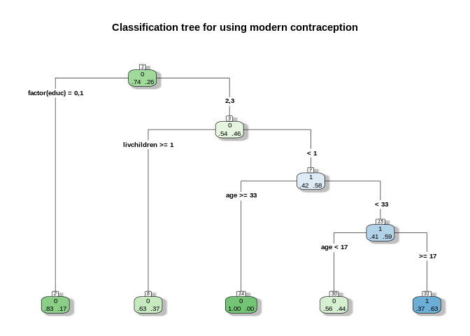
Each node box displays the classification, the probability of each class at that node (i.e. the probability of the class conditioned on the node) and the percentage of observations used at that node. From here.
predrp1<-predict(rp1, newdata=model.dat2train, type = "class")
confusionMatrix(data = predrp1,model.dat2train$modcontra )
## Confusion Matrix and Statistics
##
## Reference
## Prediction 0 1
## 0 3826 1055
## 1 210 354
##
## Accuracy : 0.7677
## 95% CI : (0.7562, 0.7788)
## No Information Rate : 0.7412
## P-Value [Acc > NIR] : 3.566e-06
##
## Kappa : 0.2475
##
## Mcnemar's Test P-Value : < 2.2e-16
##
## Sensitivity : 0.9480
## Specificity : 0.2512
## Pos Pred Value : 0.7839
## Neg Pred Value : 0.6277
## Prevalence : 0.7412
## Detection Rate : 0.7027
## Detection Prevalence : 0.8964
## Balanced Accuracy : 0.5996
##
## 'Positive' Class : 0
## We see the regression tree is performing a little better than the logistic regression on the test case using the summary below:
pred_testrp<-predict(rp1, newdata=model.dat2test, type="class")

confusionMatrix(data = pred_testrp,model.dat2test$modcontra )
## Confusion Matrix and Statistics
##
## Reference
## Prediction 0 1
## 0 947 263
## 1 61 89
##
## Accuracy : 0.7618
## 95% CI : (0.7382, 0.7842)
## No Information Rate : 0.7412
## P-Value [Acc > NIR] : 0.0434
##
## Kappa : 0.2365
##
## Mcnemar's Test P-Value : <2e-16
##
## Sensitivity : 0.9395
## Specificity : 0.2528
## Pos Pred Value : 0.7826
## Neg Pred Value : 0.5933
## Prevalence : 0.7412
## Detection Rate : 0.6963
## Detection Prevalence : 0.8897
## Balanced Accuracy : 0.5962
##
## 'Positive' Class : 0
## Linear discriminant function
Linear discriminant functions attempt to separate classes from each other using a strictly linear function of the variables. It attempts to reduce the dimensionality of the original data to a single linear function of the input variables, or the discriminant function. This is very similar to what PCA does when it creates a principal component, although in LDA, the function uses this linear transformation of the data to optimally separate classes.
In this case it performs better than the logistic regression but not as well as the regression tree.
##
## Attaching package: 'MASS'
## The following object is masked from 'package:dplyr':
##
## selectlda1<-lda(modcontra~factor(region)+scale(age)+livchildren+factor(educ), data=model.dat2train,prior=c(.74, .26) , CV=T)
pred_ld1<-lda1$class
head(lda1$posterior) #probabilities of membership in each group## 0 1
## 1 0.8153664 0.1846336
## 2 0.7387134 0.2612866
## 3 0.8673284 0.1326716
## 4 0.8080069 0.1919931
## 5 0.8976027 0.1023973
## 6 0.8387015 0.1612985ld1<-data.frame(ppmod= lda1$posterior[, 2],pred=lda1$class, real=model.dat2train$modcontra)
ld1%>%
ggplot()+geom_density(aes(x=ppmod, group=pred, color=pred))+ggtitle(label = "Probabilities of class membership on the linear discriminant function")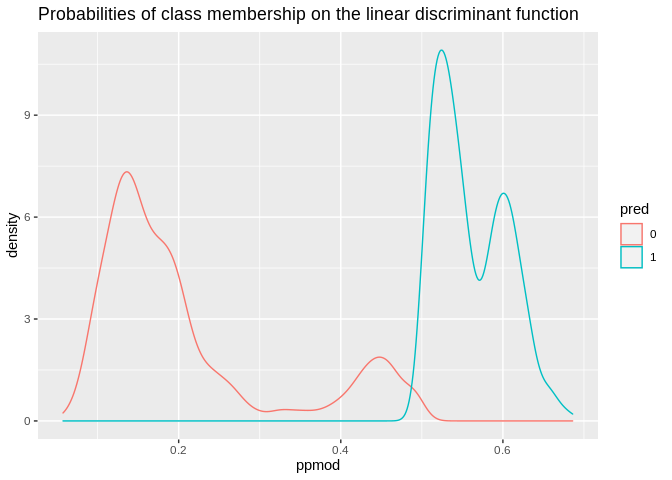
ld1%>%
  ggplot()+geom_density(aes(x=ppmod, group=real, color=real))+ggtitle(label = "Probabilities of class membership and the real class")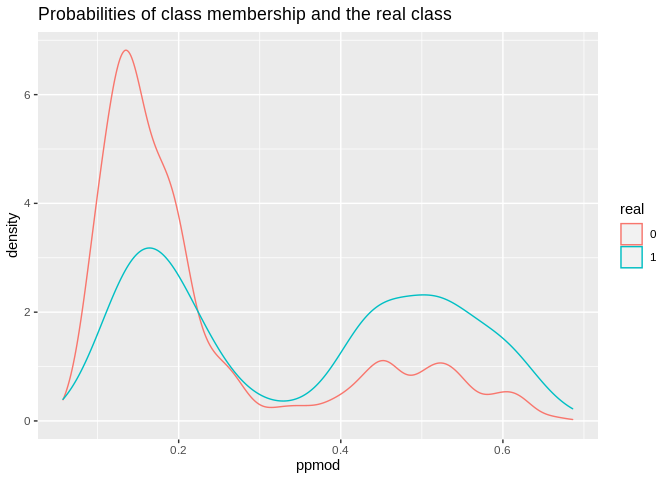
Accuracy on the training set
## Confusion Matrix and Statistics
##
##           Reference
## Prediction    0    1
##          0 3625 1000
##          1  411  409
##
##                Accuracy : 0.7409
##                  95% CI : (0.729, 0.7525)
##     No Information Rate : 0.7412
##     P-Value [Acc > NIR] : 0.5318
##
##                   Kappa : 0.2181
##
##  Mcnemar's Test P-Value : <2e-16
##
##             Sensitivity : 0.8982
##             Specificity : 0.2903
##          Pos Pred Value : 0.7838
##          Neg Pred Value : 0.4988
##              Prevalence : 0.7412
##          Detection Rate : 0.6657
##    Detection Prevalence : 0.8494
##       Balanced Accuracy : 0.5942
##
##        'Positive' Class : 0
## lda1<-lda(modcontra~factor(region)+scale(age)+livchildren+factor(educ), data=model.dat2train,prior=c(.74, .26) )
#linear discriminant function
lda1$scaling## LD1
## factor(region)2 0.4580587
## factor(region)3 0.8545973
## factor(region)4 0.3495414
## scale(age) -0.3873869
## livchildren 0.1025140
## factor(educ)1 0.4535731
## factor(educ)2 1.9263226
## factor(educ)3 2.2956187Accuracy on the test set
## Confusion Matrix and Statistics
##
##           Reference
## Prediction   0   1
##          0 906 254
##          1 102  98
##
##                Accuracy : 0.7382
##                  95% CI : (0.714, 0.7614)
##     No Information Rate : 0.7412
##     P-Value [Acc > NIR] : 0.6115
##
##                   Kappa : 0.2062
##
##  Mcnemar's Test P-Value : 1.214e-15
##
##             Sensitivity : 0.8988
##             Specificity : 0.2784
##          Pos Pred Value : 0.7810
##          Neg Pred Value : 0.4900
##              Prevalence : 0.7412
##          Detection Rate : 0.6662
##    Detection Prevalence : 0.8529
##       Balanced Accuracy : 0.5886
##
##        'Positive' Class : 0
##