library(tidyverse)
library(here)
library(sparkscolors)  # pak::pak("coreysparks/sparkscolors"), UTSA colors

source(here("R", "get_mmsa.R"))Week 1: Course Introduction and a Reproducible Workflow
Introduction
Welcome to the second semester of statistics for demographers. The first course gave you the linear model and the logic of inference, and this course takes those tools into the places demographic data actually live, which is to say complex surveys, binary and categorical outcomes, counts and rates, people nested inside places, and the same people measured over time. Every week pairs a set of methods with a real data source, and the data source for most of the semester is the CDC’s Behavioral Risk Factor Surveillance System (BRFSS), specifically the SMART metropolitan and micropolitan area (MMSA) file for 2024.
This first week is about the plumbing. I want you to leave with a working project that holds your code and data, a Quarto document that runs from top to bottom, a record of the package versions you used, and a Git repository that tracks all of it. None of this is glamorous, but I have watched enough final papers fall apart the night before they were due (sometimes my own analyses, if I’m honest) to know that the workflow matters as much as the model.
NoteThis week at a glance
The question. How do you produce an analysis that another person can check, from the data to the sentence in your paper?
By the end of this week you should be able to
- name the parts of a finished analysis (question, data, result, model, interpretation, limitations) in an example you didn’t write;
- say what each file in an analysis project is for, and which ones another reader needs to reproduce a result;
- render a Quarto document, record it with Git, and publish it, and say whether a number describes the survey respondents or the population.
Before you begin. You should know what a mean, a regression coefficient and a standard error are. The self-check in My assumptions about you will tell you whether to review anything. You don’t need to know any R yet.
Required and optional. Everything this week is required, because every later week depends on it.
The anatomy of an analysis
Before any software, here is what we’re building toward. Every analysis in this course, and every paper you write, has the same six parts. This table walks through one you’ll do yourself in weeks 2 and 3.
| Part | What it is | In the example |
|---|---|---|
| Research question | One question, specific enough to answer with data | Do adults with less education report fair or poor health more often than adults with more? |
| Data | Where the numbers come from, what one row is, and which population they describe | The 2024 BRFSS SMART file. One row is one adult who answered the survey. With the survey weights, the rows describe adults 18 and over living in households in the metro and micro areas in the file, not all U.S. adults. |
| Descriptive result | What the data show before any model | The weighted share reporting fair or poor health in each education group, with a confidence interval (week 2) |
| Model | A statement of how the outcome relates to several predictors at once | A survey-weighted logit model of fair or poor health on education, age, sex and race and ethnicity (week 3) |
| Interpretation | What the numbers mean, in units a reader cares about | “Adults without a high school diploma are about so many percentage points more likely to report fair or poor health than college graduates of the same age, sex and race and ethnicity.” |
| Limitations | What the analysis can’t tell you | Health is self-reported. The survey is a telephone survey with low response rates, and the weights only partly fix that. The data are measured at one time, so they show an association, not that more education causes better health. |
Keep this table in mind. The software we set up this week exists to make every row of it traceable: someone reading your interpretation should be able to find the code and the data that produced it.
Setup
This document only needs a few packages. here finds files relative to the project root, so the same code runs on my machine, your laptop and the course container without editing paths. The get_mmsa() function in R/get_mmsa.R reads the 2024 BRFSS MMSA file, and I’ll use it in every exercise this semester.
How the course runs
The course meets for sixteen weeks, with spring break in week 8 and final papers due in week 16. Readings for each week are listed on the syllabus. The topics are:
| Week | Topic |
|---|---|
| 1 | Course introduction; reproducible workflow with Quarto, renv, and Git; publishing to Posit Connect Cloud |
| 2 | Complex survey design, weights, replicate variance |
| 3 | Binary outcomes: logit and probit, predicted probabilities, average marginal effects |
| 4 | Comparing nested logit models (KHB); prediction and cross validation |
| 5 | Ordinal and multinomial models |
| 6 | Counts and rates: Poisson, negative binomial, offsets, zero inflation |
| 7 | Decomposition: Kitagawa and Oaxaca-Blinder |
| 8 | Spring break |
| 9 | Missing data and multiple imputation with survey designs |
| 10 | Longitudinal models: GEE, fixed effects, within-between models |
| 11 | Splines and GAMs |
| 12 | Multilevel models I: centering, random slopes, level-specific weights |
| 13 | Multilevel models II: GLMMs, growth curves, age-period-cohort models |
| 14 | Causal inference foundations: DAGs and propensity score weighting |
| 15 | Tree-based machine learning with tidymodels |
| 16 | Final papers due |
Two things are deliberately missing. Principal components no longer has its own week; if your final paper needs a composite index for places, I’ll show you how to build and defend a standardized index when we get there. Event history models are also out, because they have their own full course, and when we reach longitudinal data in week 10 I’ll point you to where that material picks up.
Reading, getting the files, and turning in homework
These are three different jobs, and they happen in three different places.
- Reading the course book. The weekly chapters are on the web at https://coreysparks.github.io/DEM7283/. You can read them in any browser, and you don’t need anything installed. Read the week’s chapter before class.
- Getting the course files. To run the code yourself, you need the course repository on your computer: the chapters’
.qmdsource files, the data indata/and the helper functions inR/. You’ll clone it with Git this week (Getting the course repository) and pull my updates each week. - Turning in homework. Each chapter ends with that week’s homework. From Homework 2 on, there are two versions: one with your own survey data and one with my data. If you’re in DEM 7283, you do the version with your own data; if you’re in DEM 5283, you choose. You do them in your own homework project, not in the course repository. You turn in two links through Canvas: the link to your rendered homework document on Posit Connect Cloud (the website that hosts it; you send it there with the Posit Publisher tool built into Positron), and the link to your GitHub repository that holds the code. Homework is due before class one week after it’s assigned.
My assumptions about you
In statistics we always make assumptions, they are often wrong, and we adapt to our mistakes daily. Here are mine about the people in this room. You took the first course (or something like it), so you know what a regression coefficient and a standard error are. You’re interested in demography or population research, as a student or as someone who works with population data. You may have used SAS, SPSS or Stata before and are curious about R, or you may be an R user from some other strange and exotic discipline who wants to see how demographers work. And you want to see how to do things, rather than being bombarded with theoretical and often unnecessary gate-keeping mathematical treatments of statistical models. There will be some equations, but every one of them is there because it helps you read the output or avoid a mistake.
This course is not a review of all of statistics, and it’s not an encyclopedic tour of the R language. I imagine the latter is on the same scale of hopelessness as the search for the Holy Grail, and I’m not falling on my sword here, folks.
Assumptions are only useful if you check them, so here’s a short self-check. It isn’t graded, and nobody sees your answers. Try each one before you open the answer. If more than one or two give you trouble, reread the regression chapters from your first course before week 3, or come see me; it’s much easier to fix now than in week 12.
- A linear regression of BMI on age (in years) gives a coefficient of 0.05 for age, with a standard error of 0.01. What does 0.05 mean, in words?
- What does the standard error of 0.01 tell you?
- The 95% confidence interval for that coefficient is 0.03 to 0.07. What does that interval say?
- Another coefficient has a p-value of 0.20. Does that show the predictor has no association with BMI?
- A data set follows 1,000 people and measures each of them in three different years, with one row per person per year. How many rows does it have? How many people?
- What’s the difference between the mean BMI of the people in a survey and the mean BMI of the population the survey was drawn from?
Answers
- Comparing people who differ in age by one year (and are the same on anything else in the model), the older person’s BMI is 0.05 points higher on average. Over ten years, that’s half a point.
- How much the coefficient would vary if we drew many samples the same way and fit the same model to each. It measures the uncertainty in the estimate that comes from sampling.
- If we repeated the sampling many times and built an interval the same way each time, 95% of those intervals would contain the true coefficient. Informally, values from 0.03 to 0.07 are consistent with the data.
- No. It says the data are consistent with no association, but they may also be consistent with an association of a meaningful size. A large p-value can come from a small sample or a noisy measure. Look at the estimate and its confidence interval, not just whether p is below 0.05.
- 3,000 rows, but only 1,000 people. The three rows for the same person aren’t independent observations, and week 10 is about what to do with that.
- The first describes the respondents, the people who happened to answer. The second describes the population. They’re only equal if the sample represents the population, which is what survey weights (week 2) are for.
Software
A vocabulary guide
You’ll meet a lot of new tools this week, and they’re easy to confuse. Here they are in one place. Come back to this table whenever a word stops making sense.
| Term | What it is | An example from this course |
|---|---|---|
| R | The program that does the computing | R 4.6 |
| Editor | The program you work in. It sends your code to R and shows you the results | Positron |
| Package | A bundle of R functions someone else wrote, which you install once and load with library() |
survey, ggplot2 |
| Function | A named piece of code that takes inputs (arguments) and returns a result | mean(), svyglm(), get_mmsa() |
| Script | A plain text file of R code, ending in .R |
R/get_mmsa.R |
| Quarto document | A file (.qmd) that mixes your writing with the code that produces the evidence, and renders to a report |
Your weekly homework |
| Project | The folder that holds one analysis and everything it needs: code, data, documents | Your homework project; the course repository |
| Git | A program that records the history of the files in a project | Each commit is one saved snapshot |
| GitHub | A website that keeps an online copy of a Git project | github.com/yourname/homework |
| Published document | A rendered Quarto document on the web, with its own link | Your homework on Posit Connect Cloud |
Why R?
We use R for everything in this course. I’ve used R for more than twenty years. I was also trained in SPSS and SAS along the way, by various mentors, some of whom tried to get me to learn general-purpose languages like Delphi (of all things), Perl or Basic, and I’ve been chastised for not knowing the depths of Python. But R is a nimble and rigorous platform to do demography, and my top three reasons for teaching it are these:
- It’s free. Why should we pass more costs along to people, especially students? Being free also makes R code accessible to people all over the world, including the colleagues at statistical offices and universities we collaborate with.
- It’s where new methods show up first. The R ecosystem has more than 20,000 packages on CRAN alone, and many of them represent the leading edge of data analysis, visualization and data science. Methods for survey data, small area estimation and demographic analysis often appear in R years before they show up in commercial software.
- It has a supportive community. There are debates about how friendly some R users are to newcomers, but after twenty-plus years in the R community I’ve personally helped hundreds of users and been helped by many others. The open source nature of R lends itself to sharing ideas and code.
If you’re coming to R from SAS, there is no data step and there are no procs. Kleinman and Horton (2014) is a very useful crosswalk between the two programs. If you’re coming from SPSS and you’ve been using the point-and-click method, be prepared for a steep learning curve. If you’ve been writing SPSS syntax, you’re at least used to writing code. Stata users have fewer published crosswalks, but I have always thought Stata and R were very similar in spirit, and most of what you know about svyset and margins carries over directly to the survey and marginaleffects packages we’ll use.
What to install
You need three programs: R, Positron and Git. The Before the First Class page has the step-by-step instructions, so here I’ll just say what each one is for.
- R (the current release, 4.6.x as I write this) does the computing. Install it first. On Windows, also install Rtools (the version that matches your R release), because it gives you the C++ and Fortran compilers that some packages need.
- Positron is the editor you’ll work in, and it’s what I use in class. It’s made by Posit, the company that makes RStudio, and if you’ve used RStudio before, most of it will feel familiar. Install it after R, from https://positron.posit.co/download. It comes with Quarto and with the Posit Publisher extension we’ll use to share homework, so you don’t need to install either one separately.
- Git keeps the history of your work, and the Git section below walks you through installing it and setting up GitHub.
The first time you open Positron, it finds your R installation and starts an R session in the Console. If it doesn’t, click the interpreter button at the top right of the window and choose R. The window has four main areas: an editor where you write code (run the current line or a highlighted block with Ctrl-Enter, or Cmd-Enter on a Mac), the Console, where results, warnings and errors show up, a Variables pane listing the objects you’ve created, and panes for plots, help and the files in your project. In R a warning doesn’t necessarily mean something went wrong. It’s R’s polite way of telling you to pay attention. An error does mean something went wrong, very often a missing ) or a misspelled name. I routinely type lenght for length, and R routinely tells me about it.
If you would rather not install anything, the course repository includes a development container. Opening the repository in a GitHub Codespace, or in VS Code with the Dev Containers extension, gives you R, Quarto and the BRFSS data already in place. This is also a nice fallback when a package refuses to compile on your laptop the week a homework is due.
Note
Some exercises also have Python versions. They are there for students who work in Python, but R is the primary tool in this course, and a few of the methods we use (survey-weighted multinomial models and KHB comparisons, for example) don’t have good Python equivalents.
Packages and functions
R keeps its functions in packages, and we will install a lot of them. Most live on CRAN, the Comprehensive R Archive Network, which is the official repository. Others live on Bioconductor, R-universe or GitHub, especially while they’re being developed (my sparkscolors package is one of those). CRAN also organizes packages into Task Views, thematic lists maintained by people who work in an area. There isn’t one for demography, but the Official Statistics and Survey Statistics, Social Sciences and Spatial views cover most of what we do, and the ctv package can install every package in a view at once.
You install a package once, but you load it with library() every time you start a new session.
install.packages("survey")   # once
library(survey)              # every session

update.packages(ask = FALSE) # every so often, for bug fixes and new features
Installing the packages for this course one at a time would take you most of an afternoon, so I wrote a script that does it for you (the setup page walks through the whole installation). Run this once, before our second meeting:
source("https://raw.githubusercontent.com/coreysparks/DEM7283/master/install_first_7283.R")source() downloads the file and runs every line in it. Read it first, because you should never run code from the internet that you haven’t looked at, mine included. It’s short. It installs pak, a faster installer that pulls prebuilt binaries from CRAN and can also install from GitHub, and then hands pak the list of packages we’ll use this semester, grouped by the week they show up, plus sparkscolors from my GitHub. Anything you already have is skipped, so if it stops partway through (a dropped Wi-Fi connection, a laptop going to sleep), just run it again and it picks up where it left off. The first run takes a while. Go get a coffee.
If you’re on Windows, the script will also tell you if it can’t find Rtools. You won’t need Rtools until week 12, when brms has to compile models in C++, but it’s much less painful to install it now than the night before a homework is due.
Different packages sometimes use the same name for different functions. Base R’s stats package has a lag() for time series, and dplyr has a lag() that works on vectors and takes different arguments. Whichever package you loaded last wins, and R prints a message about the conflict when you load it. When you want to be sure which one you’re getting, use the package::function() form, like stats::lag() or dplyr::lag(). You’ll see me do this throughout the course, and you’ll also see it inside the helper functions in R/, where it means the function works without loading the whole package. Package authors deal with this too: car::recode() was renamed car::Recode() so it wouldn’t collide with dplyr::recode(), because the two are so often used in the same analysis.
A function is just a bit of code with arguments. Some arguments are required, and some have defaults you can change. Here is a function that finds the mean of a vector:
mymean <- function(x, na.rm = FALSE) {
  if (na.rm) x <- x[!is.na(x)]
  sum(x) / length(x)
}

mymean(c(1, 2, 3))
#> [1] 2mymean(c(1, 2, NA, 3))#> [1] NAmymean(c(1, 2, NA, 3), na.rm = TRUE)#> [1] 2The na.rm = FALSE default means the function returns NA if any value is missing, which is exactly what base R’s mean() does, and it’s one of the most common surprises for new R users. Many R functions either fail or quietly drop cases when there are NAs, so check the help file to see what a function does with missing values. In general, if you find yourself writing the same code over and over, write a function. Save it in a script and source() it, the way the exercises source() the files in R/. If you get serious about it, put it in a package (Wickham and Bryan 2023).
Getting help
I wish I had a nickel for every time I ran into a problem trying to do something in R. Here is where I look:
- If you know the function,
?svyglmopens its help page. Read the whole thing at least once. The help page lists every argument (this is where the alternative specifications of a model live), gives the citations for the methods, and ends with examples you can run. - If you don’t know the function,
??"survey design"searches the help pages of every installed package. - Package vignettes (
browseVignettes("survey")) are longer tutorials written by the authors, and they’re often the best documentation there is. - Stack Overflow and Cross Validated have answers to most questions you’ll have. Many answers are snarky, wrong, or written for an old version of a package, so caveat emptor.
- AI assistants can be genuinely helpful for explaining an error message or a block of code. They also make up function arguments with total confidence. Run what they give you, read the help page for anything unfamiliar, and never paste restricted data into one.
- Your local R guru or user group. There may be an R user just down the hall. Even after twenty years I learn something every time I talk to someone about how they use R.
When you ask a person for help, include a reproducible example: the smallest bit of code and data that shows the problem. The reprex package makes one for you. Half the time, building the example is how you find the bug.
Last, there is almost always more than one way to do something in R. Reading a CSV file can be done by a handful of functions in different packages. If someone tells you there’s only one way to do something in R, they’re usually wrong.
Data formats
R reads and writes its own formats and those of every other statistics package. The native formats are .rds, which holds a single object (saveRDS() and readRDS()), and .RData, which can hold several (save() and load()). I prefer .rds, because you choose the name of the object when you read it back in, and that’s what get_mmsa() uses for its cached copy of the BRFSS. Text files are read with read.csv() or readr::read_csv(). The haven package reads and writes SAS (.sas7bdat and transport .xpt files), Stata (.dta) and SPSS (.sav and .por) files, and it’s what reads the BRFSS transport file and the DHS Stata file we’ll use.
library(haven)
dhs <- read_dta(here("data", "ZZIR62FL.DTA"))
brfss_raw <- read_xpt(unzip(here("data", "MMSA2024_XPT.zip"), exdir = tempdir()))
R also has packages for Excel (readxl), JSON, shapefiles and other spatial formats (sf), and SQL databases (DBI), and for talking to Mplus, Stan and various GIS programs.
A reproducible workflow
When I say an analysis is reproducible, I mean that another person can trace how your evidence supports your conclusion: from the sentence in your paper, to the number behind it, to the code that computed it, to the data it came from. That other person is often you, six months from now, with no memory of what you did. The test is simple: can someone take your files, run them, and get the same numbers? The tools below are just ways of making the answer yes. In practice that takes four pieces:
- a project that keeps code, data and output together,
- a Quarto document that runs from the first line to the last with no hidden steps,
- renv, which records the package versions you used, and
- Git, which records every change you made and lets you share the whole thing on GitHub.
I’ll take these one at a time, and then show you how to put the rendered document on the web with Posit Connect Cloud, which isn’t part of reproducibility but is how you’ll share your homework.
Projects and file paths
The fastest way to break someone else’s code is a line like read.csv("C:/Users/ozd504/OneDrive/projects/data.csv"). It works on exactly one computer in the world. In Positron, a project is simply a folder: you open it with File > Open Folder, and R starts in that folder. The here package finds the top of the project (it looks for markers like a .git folder or the .Rproj file at the top of this repository) and builds paths from there.
here()#> [1] "/Users/ozd504/github/DEM7283"here("data", "MMSA2024_XPT.zip")#> [1] "/Users/ozd504/github/DEM7283/data/MMSA2024_XPT.zip"Your output will show a different root than mine, and that is the point: the second line finds the data file no matter where you cloned the repository. Every exercise this semester uses here() for file paths, and I’d like your homework to do the same.
Quarto documents
A Quarto document (.qmd) mixes prose and code. The YAML header at the top controls the output, and each code chunk carries its options in #| comments. A minimal homework document looks like this:
---
title: "Homework 1"
author: "Your Name"
format:
  html:
    embed-resources: true
execute:
  echo: true
---

## Setup

```{r}
#| label: setup
library(tidyverse)
library(here)
```
The embed-resources: true option packs the figures and styles into a single, self-contained HTML file, so you can submit or share one file. (Older tutorials call this option self-contained: true. Quarto renamed it in version 1.4, and the old name still works but prints a deprecation warning.) Render the document with the Render button, with quarto render homework1.qmd in the terminal, or with quarto::quarto_render("homework1.qmd") from R. Rendering starts a fresh R session, so if your document only works because of something you ran in the console an hour ago, rendering will tell you. That’s the feature, not a bug.
Recording package versions with renv
Packages change. A function gets a new default, an argument gets renamed, or a package disappears from CRAN, and code that ran last spring stops running. renv gives each project its own package library and writes the exact versions into a lockfile, renv.lock, which you commit along with your code.
renv::init()      # once per project: create the project library and lockfile
renv::snapshot()  # after you install or update packages: record the versions
renv::status()    # check whether the lockfile and library agree
renv::restore()   # on a new machine: install the versions in renv.lock
The usual rhythm is to install what you need, get the analysis working, run renv::snapshot(), and commit renv.lock. When a classmate (or I) clone your repository, renv::restore() rebuilds your library.
The course repository works the same way. When I rendered these weekly documents, I snapshotted the packages into the renv.lock file at the top of the repository, so the lockfile is a record of exactly which version of every package produced the output you’re reading. If you clone the repository and open the project, renv starts itself (that’s what the .Rprofile file is for) and tells you the project library is out of sync. Run this once:
renv::restore() # install the versions I used for the course materialsSo why bother with the install script at all? The two do different jobs. The script puts current versions of the course packages in your own R library, which is what you want for your homework and your own projects. renv::restore() gives the course project its own library with my versions, which is what you want when one of my examples gives you a different number than it gave me, or throws an error I never saw. Nine times out of ten that’s a package update, and restoring the lockfile is the fastest way to find out. And renv keeps a cache of everything it installs, so after the first restore, renv::init() in your own homework projects goes quickly.
Version control with Git and GitHub
If you’ve ever had a folder with paper_final.docx, paper_final2.docx and paper_final_REALLY_final_CS_edits.docx in it, you already understand the problem version control solves. You want to keep the old versions in case you need them, but you also want to know which file is the current one and what changed between them. Git does this for a whole project folder. Whenever you reach a point worth keeping, you take a snapshot of the project, called a commit, with a short note about what changed. Git stores every snapshot, so you can see the history of any file, compare two versions, or go back to an old one, and the folder itself only ever holds the current version of each file. No more _final2.
GitHub is a website that keeps a copy of your Git project online. That gives you a backup, a way to move your work between computers, and a link you can send to someone (me, for your homework) so they can see your code. Git is the program on your computer, and GitHub is one of several places to store what Git records. You can use Git without GitHub, but not the other way around, at least not in any useful way.
Most of you have never used either, and that’s fine. Setting it up takes about an hour, once, and after that the everyday use is a few clicks. Most data analysts I know learned Git the way they learned R, by needing it, and after a month they stopped thinking about it. I’ll go through the setup step by step. Do the steps in order and don’t skip any, because each one depends on the one before.
A few words you’ll need
Git has its own vocabulary, and its error messages assume you know it.
- Repository (or repo): a project folder that Git is tracking. On your computer, it’s an ordinary folder with a hidden
.gitfolder inside, where Git keeps the history. Leave the.gitfolder alone. On GitHub, a repository is the online copy of that folder. - Commit: a snapshot of the files you chose, with a message describing the change. The list of commits is the history.
- Stage: choose which changed files go into the next commit. You don’t have to commit everything you changed at once.
- Push: send your new commits from your computer up to GitHub.
- Pull: bring new commits down from GitHub to your computer.
- Clone: download a complete copy of a repository from GitHub, history and all, as a new folder on your computer.
- Remote: the copy of the repository somewhere else, which for us is always GitHub. Git calls it
origin. - Branch: a separate line of history. Every repository starts with one, usually called
main(older repositories, like the course repository, call itmaster). We’ll only use one branch this semester.
Step 1: Create a GitHub account
- Go to https://github.com and click Sign up.
- Use an email address you’ll still have after you graduate. Your repositories become part of your professional record, and you don’t want to lose access to them when your UTSA email goes away. You can add your UTSA address as a second email later, under Settings > Emails.
- Choose your username with some care. It’s in the web address of everything you put on GitHub (
https://github.com/yourname/homework), and future employers and collaborators will see it. Your name, or something close to it, is a good choice. Mine iscoreysparks. - Pick the Free plan. Free accounts can have as many public and private repositories as you like, which is all you need. Students can also apply for the GitHub Student Developer Pack with a school email, but nothing in this course needs it.
Step 2: Install Git
Git is a separate program. Positron uses it, but doesn’t include it.
- Windows: download Git for Windows from https://git-scm.com/downloads/win and run the installer. It asks a lot of questions, and the defaults are fine for all but two of them. When it asks you to choose the default editor used by Git, pick Notepad (or VS Code, if you have it) instead of Vim. Vim is a powerful editor, and it’s famously hard to get out of if you’ve never used it. And when it asks about the name of the initial branch, choose Override the default branch name and type
main. - macOS: open the Terminal app (in Applications > Utilities), type
git --versionand press Return. If Git isn’t installed, macOS offers to install the command line developer tools, which include it. Click Install. If you installed them on the setup page, Git is already there. - Linux: install the
gitpackage with your distribution’s package manager.
Checking that it worked means meeting the Terminal. Positron has a Console and a Terminal side by side, as tabs in the panel at the bottom of the window. The Console runs R code. The Terminal runs commands for your computer’s operating system, and Git commands go there. If you type a Git command into the R Console, R will tell you, quite rightly, that it has no idea what you mean. If you don’t see the Terminal tab, choose View > Terminal.
Close Positron completely and open it again, so it notices the new program, then click into the Terminal and type:
git --versionYou should see something like git version 2.51.0. The exact number doesn’t matter. If you see command not found or 'git' is not recognized, restart Positron and try again. If it still fails, Git didn’t install, so run the installer again.
Step 3: Tell Git who you are
Every commit records who made it, so before your first commit Git needs your name and email. Run this in the R Console, with your own name and the email you used for GitHub:
library(usethis)
use_git_config(user.name = "Your Name",
               user.email = "the-email-you-used-for-github@example.com")
git_default_branch_configure()   # call the first branch of new repositories "main"
NoteCode explanation: telling Git who you are
usethis is a package of helper functions for setting up R projects. It handles most of the Git setup from R, so you don’t have to learn the Git commands for these one-time jobs.
use_git_config() saves your name and email in Git’s settings on your computer (a file called .gitconfig in your home folder). Those settings apply to every project, so you do this once per computer, not once per project. Use the same email you used for your GitHub account. GitHub matches commits to accounts by email, so with a different one, your commits won’t show up as yours.
git_default_branch_configure() tells Git to name the first branch of every new repository main, which is what GitHub expects. If you already chose main in the Windows installer, running it again does no harm.
Step 4: Connect your computer to GitHub with a token
When you push, GitHub needs to know it’s really you, and it won’t accept your GitHub password for that. Instead, you make a personal access token (PAT), a long random string that works like a password for Git only, and that you can cancel at any time without changing your real password. Run these two lines in the Console, one at a time:
usethis::create_github_token()   # opens GitHub in your browser
gitcreds::gitcreds_set()         # paste the token when asked
NoteCode explanation: personal access tokens
create_github_token() opens the GitHub page for making a new token, with the permissions R needs already checked. Change two things on that page:
- Note: a name for the token, like “laptop DEM 7283”, so later you’ll know which computer it belongs to.
- Expiration: GitHub suggests 30 days, which means the token would stop working in the middle of the semester. Choose Custom and pick a date after the semester ends.
Scroll to the bottom and click Generate token. Then copy the token right away. It starts with ghp_, and GitHub shows it to you only once. If you close the page before copying it, no harm done; just make another one.
gitcreds_set() then asks for the token in the Console (? Enter password or token:). Paste it and press Enter. It saves the token in your operating system’s password store (the Credential Manager on Windows, the Keychain on macOS), where Git finds it every time you push. That’s also why you never put the token in a script, a .qmd file or an email: anyone who has it can change your repositories.
Now check everything you’ve done so far:
usethis::git_sitrep()git_sitrep() (short for “situation report”) prints your Git settings and whether R can reach GitHub with your token. Read it from the top. Your name, email and default branch should be the ones you set, and in the GitHub section it should show your username and say the personal access token was <discovered>. Anything marked with a red ✖ tells you which step to go back to.
Step 5: Put your homework project under version control
This is the step you’ll repeat for each new project: your homework project now, and your final paper later. Open the project folder in Positron first (File > Open Folder), then run these two lines in the Console, one at a time, and answer the questions they ask:
usethis::use_git()      # start tracking this project with Git
usethis::use_github()   # make a matching repository on GitHub and push to it
NoteCode explanation: use_git() and use_github()
use_git() turns the project folder into a Git repository (that’s when the hidden .git folder appears). It lists the files in the project and asks whether it’s OK to commit them. The answers are in a different order every time, so read them and pick the one that means yes. That makes your first commit.
use_github() creates a new, empty repository on GitHub with the same name as your project folder, connects your project to it (as the remote called origin), pushes your first commit, and opens the new repository in your browser. Refresh that page whenever you want to see what’s on GitHub.
The new repository is public by default, so anyone can see it. That’s the simplest choice for homework, because I can open the link you submit. If you’d rather keep it private, run usethis::use_github(private = TRUE) instead. Then, on the repository’s GitHub page, go to Settings > Collaborators, click Add people and add me (coreysparks), or I won’t be able to see your work.
You only run these two functions once per project. From then on, you use the everyday cycle below.
Step 6: The everyday cycle: commit, push, pull
Once the project is set up, the work goes like this. You edit files, run code and render your document. When you get to a point worth keeping (a section works, a figure looks right, you’re stopping for the night), you commit the files you changed with a message, and then you push the commit to GitHub. There’s no rule about how often. I commit whenever I’d be annoyed to lose what I just did, which is several times a session.
You can do this by clicking or by typing. Use whichever you like, because they do exactly the same thing.
By clicking, in Positron:
- Click the Source Control icon in the Activity Bar on the left. It looks like three small circles joined by lines, and a number on it tells you how many files have changed.
- Under Changes, you’ll see each changed file. Click a file to see what changed, with the old version on the left and the new one on the right.
- Hover over a file and click the + to stage it. It moves to a Staged Changes list. Stage every file you want in this commit.
- Type a message in the box at the top, like “Add BMI table by age group”.
- Click Commit.
- Click Sync Changes (it appears where the Commit button was) to send the commit to GitHub. Sync also pulls any new commits from GitHub first.
Next to each file in the list, a letter tells you what happened to it: M for modified, U for a new file Git isn’t tracking yet (untracked), D for deleted.
By typing, in the Terminal:
git status
git add homework1.qmd renv.lock
git commit -m "Add BMI table by age group"
git push
NoteCode explanation: the everyday Git commands
Each line is a Git command, typed in the Terminal (not the R Console) from inside your project folder. Positron’s Terminal starts in the folder you have open, so you don’t need to move anywhere first.
git statuslists the files that have changed since your last commit, and which of them are staged. It doesn’t change anything, so run it whenever you’re not sure what’s going on.git add homework1.qmd renv.lockstages those two files. You can list as many files as you want, or typegit add .to stage everything that changed (the.means “this folder”). If you use., rungit statusfirst so you know what you’re staging.git commit -m "Add BMI table by age group"makes the commit. The message goes in quotes after-m. If you leave out-mand the message, Git opens a text editor and waits for you to type one (see “If something goes wrong” below if that happens).git pushsends your new commits to GitHub.
Two more you’ll use: git pull brings down new commits from GitHub, and git log --oneline lists your commits, newest first, one per line.
Commit messages are for future you. “Add BMI table by age group” tells you what happened. “stuff” tells you nothing, and you’ll discover that at exactly the moment you’re trying to find which commit broke your code. Write a short description of what the commit does, in under about 60 characters.
If you work on more than one computer, pull when you start and push when you stop. That keeps the copies the same, and it’s the best way to avoid the one Git problem that’s genuinely annoying, the merge conflict (see below).
Getting the course repository
The course materials (these chapters, the data and the functions in R/) are in a GitHub repository too, https://github.com/coreysparks/DEM7283, and you’ll want a copy on your computer. Cloning downloads the whole thing and keeps it connected to GitHub, so you can get my updates each week with a pull.
usethis::create_from_github("coreysparks/DEM7283", fork = FALSE)
NoteCode explanation: create_from_github()
create_from_github() clones a repository and opens it as a project. The first argument is the repository’s owner and name, "owner/name", the same as the end of its web address. fork = FALSE says you want a copy to read and run, not your own version of the repository on GitHub (that’s a fork, and you don’t need one). The folder goes somewhere easy to find, like your Desktop or home folder. Add destdir = "path/to/folder" to choose the place yourself.
If you’d rather click: in Positron, open the Command Palette (Ctrl+Shift+P on Windows, Cmd+Shift+P on a Mac), type Git: Clone, paste the same address and choose a folder.
I’ll add and fix things in the course repository during the semester. To get my changes, open the course project and pull (Sync Changes in Positron’s Source Control view, or git pull in the Terminal). Do it at the start of each week.
One rule keeps this painless: don’t edit the files in the course repository. If you change one of my files and I change the same file, Git can’t bring down my version without overwriting yours, so it stops and complains. Copy what you need (a chapter’s .qmd file, or a function from R/) into your own homework project, and work on the copy. If you’ve already changed something by accident and a pull fails, run git restore . in the Terminal inside the course project. That throws away your changes to my files (it leaves new files you added alone), and then the pull will work.
What doesn’t belong in Git
Git is for the files you write: code, Quarto documents, renv.lock and other small text files. Some things should stay out:
- Data. Data files are usually big, and GitHub rejects any single file over 100 MB. Your repository is also public unless you made it private. You don’t lose anything by leaving data out, because
get_mmsa()downloads the BRFSS file from the CDC into your project’sdata/folder whenever it isn’t already there. - Restricted data, ever. If you use restricted data for your paper (and some of you will), it never goes in a repository, public or private. Your data use agreement almost certainly forbids putting it on someone else’s server, and once a file has been pushed, removing it from the history is hard to do completely.
- Files R makes for you. The
renv/library/folder,.Rhistoryand.RDatacan all be rebuilt from your code. - Passwords, API keys and tokens, including your Census API key and your GitHub token.
You tell Git which files to leave alone by listing them in a file called .gitignore at the top of the project. use_git() and renv::init() already add the R and renv files to it. Add the data folder yourself:
usethis::use_git_ignore("data/")
NoteCode explanation: .gitignore
.gitignore is a plain text file with one pattern per line. Git acts as if anything matching a pattern isn’t there: it doesn’t show up in git status or the Git pane, and git add . won’t stage it. use_git_ignore("data/") adds the line data/ to the file, which means “the folder called data and everything in it.” You can open .gitignore and edit it like any other text file.
Ignoring only applies to files Git isn’t already tracking. If you committed a file before you ignored it, adding it to .gitignore doesn’t take it out of the repository, so set this up right after use_git(), before you commit anything else.
Warning
Before every commit, look at the list of files you’re staging. Those two seconds are how you catch a data file, or a file with a password in it, before it goes to GitHub, which is much easier than getting it back off.
If something goes wrong
'git' is not recognizedorgit: command not found. Git isn’t installed, or your editor was already open when you installed it. Restart the editor. If that doesn’t fix it, reinstall Git (step 2).Please tell me who you arewhen you commit. Git doesn’t have your name and email yet. Do step 3.Git asks for a username and password when you push, or says
Authentication failed. Your token is missing or has expired. Make a new one and store it (step 4). Don’t type your GitHub password here; it won’t work.fatal: not a git repository. Either the Terminal isn’t in your project folder, or the project isn’t a Git repository yet. Open the project in your editor, so the Terminal starts in the right place, or runusethis::use_git().Your push is rejected with
Updates were rejected because the remote contains work that you do not have locally. GitHub has commits you don’t have yet, usually because you pushed from another computer or edited a file on the GitHub website. Pull first, then push.A pull stops with
CONFLICT (content): Merge conflict in .... The same lines of the same file changed in both copies, and Git wants you to decide which version to keep. Open the file, and you’ll find the conflict marked like this:<<<<<<< HEAD your version of the lines ======= the version from GitHub >>>>>>> origin/mainEdit that block so it says what you want, delete the three marker lines, and save the file. Then stage it and commit, and that commit finishes the job. Positron highlights the conflict and puts buttons above it (Accept Current Change, Accept Incoming Change, Accept Both Changes), so you can usually click instead of editing by hand. If the conflict is a mess, or it’s in a file you don’t recognize, stop and ask me before you try anything clever.
You ran
git commitwithout-mand you’re stuck in a strange editor. That’s probably Vim. Press Esc, type:q!and press Enter. That quits without committing, and you can commit again with-m "your message".You pushed a file you shouldn’t have (data, a password). Don’t try to fix it with commands you found online, because some of them make it worse. If it’s a password, key or token, cancel or change it right away wherever it came from, since anyone could have seen it. Then come see me.
For anything beyond this, Jenny Bryan’s Happy Git and GitHub for the useR is written for exactly our situation, R users who need Git, and much of the setup above follows it.
The course data
Most examples this semester use the 2024 BRFSS SMART MMSA file. The BRFSS is a telephone survey of adults that every state runs with the CDC, and the SMART program (Selected Metropolitan/Micropolitan Area Risk Trends) reweights the respondents who live in metro and micro areas with enough respondents, so we can make estimates for places like San Antonio and not just for Texas. The data and documentation are on the CDC SMART page, and you’ll want the variable layout and the calculated variables codebook open whenever you recode anything.
get_mmsa() reads the file. The first time you run it, it uses the zip file in data/ (or downloads it from the CDC if the zip isn’t there), cleans up the variable names, and saves a copy as an .rds file, so later reads take a few seconds instead of a minute.
brfss <- get_mmsa(2024)
dim(brfss)
#> [1] 230630 173The variable names in the raw file are a mix of plain names (GENHLTH) and calculated variables that start with an underscore (_BMI5). get_mmsa() lower-cases everything and drops the underscores, so _STSTR becomes ststr. Keep that in mind when you read the codebook.
overview <- brfss |>
  summarise(respondents = n(),
            places = n_distinct(mmsa),
            strata = n_distinct(ststr),
            weighted_adults = sum(mmsawt))
overview
#> # A tibble: 1 × 4
#> respondents places strata weighted_adults
#> <int> <int> <int> <dbl>
#> 1 230630 126 1198 157366492.So the file has 230,630 respondents in 126 metro and micro areas, and the weights add up to about 157 million adults. That last number is the first hint of what week 2 is about: each respondent stands in for a different number of people, and those numbers are not small.
brfss |>
  ggplot(aes(x = mmsawt)) +
  geom_histogram(bins = 60, fill = utsa_cols("midnight"), colour = "white") +
  scale_x_log10(labels = scales::label_comma()) +
  labs(x = "MMSA final weight (_MMSAWT)", y = "Respondents")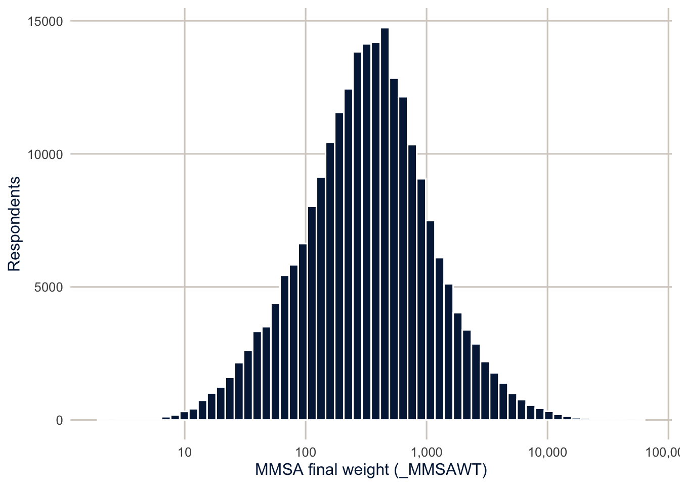
The weights run from about 2 to more than 58,200. A respondent with a weight of 1,000 represents 1,000 adults in their metro area, and a respondent with a weight of 20 represents 20. If we ignore that, we are treating every respondent as if they count the same, and they don’t.
Here is the same idea for the six Texas areas in the file, comparing the number of respondents with the number of adults they represent.
tx_counts <- brfss |>
  filter(str_detect(mmsaname, ", TX")) |>
  mutate(place = str_remove(mmsaname, ", TX.*")) |>
  group_by(place) |>
  summarise(respondents = n(),
            adults_represented = sum(mmsawt)) |>
  mutate(adults_per_respondent = adults_represented / respondents) |>
  arrange(desc(adults_represented))

knitr::kable(tx_counts, digits = 0, format.args = list(big.mark = ","))| place | respondents | adults_represented | adults_per_respondent |
|---|---|---|---|
| Houston-Pasadena-The Woodlands | 1,751 | 5,799,251 | 3,312 |
| Dallas-Plano-Irving | 1,639 | 4,326,227 | 2,640 |
| San Antonio-New Braunfels | 1,446 | 2,116,265 | 1,464 |
| Fort Worth-Arlington-Grapevine | 1,102 | 2,050,314 | 1,861 |
| Austin-Round Rock-San Marcos | 1,071 | 2,029,166 | 1,895 |
| Beaumont-Port Arthur | 508 | 302,437 | 595 |
The big metros get more respondents, but not in proportion to their size. Each Houston respondent stands in for about 3,312 adults on average, and each San Antonio respondent for about 1,464. So a San Antonio respondent counts for less than half as much as a Houston respondent when we add things up. Next week we’ll take this seriously and use the weights and the design of the survey to get estimates, and standard errors, that describe the population and not just the sample.
TipReading the result: a right and a wrong interpretation
Right: “The 2024 file has 1,446 respondents in San Antonio, and their weights add up to about 2,116,265 adults, the estimated adult population the respondents represent.”
Wrong: “The BRFSS surveyed 2,116,265 adults in San Antonio.” The number of people surveyed is the number of rows. The sum of the weights is the number of people those respondents stand in for. Mixing the two up is the most common mistake people make with survey data, and week 2 shows what it does to a standard error.
A refresher on describing data
The first course covered descriptive statistics, but it’s worth a quick tour of how I do this in R, because these are the tools you’ll use every week. One warning before we start: everything in this section ignores the survey weights. These are descriptions of the sample, and that’s fine for getting to know a data file and checking recodes, but they are not estimates for the population. Week 2 fixes that.
A first look at a variable
BMI is stored with two implied decimal places (a value of 2734 means 27.34), and self-rated health is coded 1 (excellent) to 5 (poor), with 7 and 9 for “don’t know” and “refused.” Always check the codebook for codes like these before you summarize anything.
brfss <- brfss |>
  mutate(bmi = bmi5 / 100,
         genhlth = if_else(genhlth %in% 1:5, genhlth, NA_real_),
         sex = factor(sexvar, levels = 1:2, labels = c("Male", "Female")),
         agec = factor(ageg, levels = 1:6,
                       labels = c("18-24", "25-34", "35-44", "45-54", "55-64", "65+")))
summary() is the fastest first look. For a numeric variable it gives the five-number summary plus the mean, and it counts the NAs, and for a factor it gives a frequency table.
summary(brfss$bmi)#> Min. 1st Qu. Median Mean 3rd Qu. Max. NAs
#> 12.08 24.03 27.37 28.38 31.47 99.84 23135summary(brfss$agec)#> 18-24 25-34 35-44 45-54 55-64 65+
#> 16424 28818 33222 34194 39429 78543I find this very useful when I’m first exploring a data file, because it shows the minimum and maximum right away, and that’s where impossible values and leftover missing codes show up. Alternatives that summarize a whole data frame include skimr::skim() and Hmisc::describe().
The mean and median need to be told what to do with missing values, and the variance and standard deviation do too.
mean(brfss$bmi)#> [1] NAmean(brfss$bmi, na.rm = TRUE)#> [1] 28.37926median(brfss$bmi, na.rm = TRUE)#> [1] 27.37sd(brfss$bmi, na.rm = TRUE)#> [1] 6.519392Frequency tables
table() counts the observations in each category, and with two variables it makes a cross-tabulation. One of my favorite things in base R is the I() function, which evaluates whatever is inside it, so you can build a binary variable on the fly:
table(brfss$genhlth, useNA = "ifany")#>
#> 1 2 3 4 5 <NA>
#> 34690 75416 77808 32400 9690 626table(obese = I(brfss$bmi >= 30), brfss$sex)#>
#> obese Male Female
#> FALSE 71198 69188
#> TRUE 32110 34999I(brfss$bmi >= 30) is TRUE for anyone with a BMI of 30 or more, and table() counts the TRUEs and FALSEs for men and women. prop.table() turns counts into proportions, and xtabs() does the same job with a formula interface, which we’ll use next week to make weighted tables.
The tidyverse
Most of the code in this course uses the tidyverse (Wickham et al. 2019), a collection of packages that share a philosophy about how data and code should fit together. The two workhorses are dplyr, for manipulating data, and ggplot2, for graphics. Both are covered in depth in R for Data Science (Wickham et al. 2023), so here I’ll just show how they show up in my own workflow.
dplyr is built around a small number of verbs: filter() keeps rows, select() keeps columns, mutate() makes new variables, group_by() splits the data into groups (the same idea as SAS’s by processing), and summarise() collapses each group to a row. The pipe, |>, passes the result of one step to the next, so you only name the data once, and you don’t need $ to get at the variables. I often say that I can do something in about 10 lines of R that takes 50 in SAS, and with dplyr it’s fewer still.
brfss |>
  filter(!is.na(bmi), !is.na(sex)) |>
  mutate(obese = bmi >= 30) |>
  group_by(sex, agec) |>
  summarise(n = n(),
            mean_bmi = mean(bmi),
            pct_obese = 100 * mean(obese),
            .groups = "drop")
#> # A tibble: 12 × 5
#> sex agec n mean_bmi pct_obese
#> <fct> <fct> <int> <dbl> <dbl>
#> 1 Male 18-24 8511 25.7 18.3
#> 2 Male 25-34 13753 27.8 27.7
#> 3 Male 35-44 14966 28.8 33.5
#> 4 Male 45-54 14900 29.5 37.6
#> 5 Male 55-64 17462 29.3 37.3
#> 6 Male 65+ 33716 28.1 28.5
#> 7 Female 18-24 6023 25.9 21.4
#> 8 Female 25-34 11564 28.5 34.5
#> 9 Female 35-44 14582 29.2 37.4
#> 10 Female 45-54 15267 29.6 39.9
#> 11 Female 55-64 18287 29.1 37.6
#> 12 Female 65+ 38464 27.6 29.4That reads almost like a sentence: take the BRFSS, keep people with BMI and sex recorded, flag obesity, group by sex and age, and give me the count, the mean BMI and the percent obese in each group. across() applies the same summary to several variables at once:
brfss |>
  group_by(sex) |>
  summarise(across(c(bmi, genhlth), \(x) mean(x, na.rm = TRUE)))
#> # A tibble: 2 × 3
#> sex bmi genhlth
#> <fct> <dbl> <dbl>
#> 1 Male 28.4 2.57
#> 2 Female 28.4 2.62Basic ggplot
A ggplot() has three parts. The first is the data and the aesthetic mapping, set with aes(), which says which variables go on which axes (and, later, which ones set color, fill or shape). The second is one or more geometries, which say how to draw the data. The third is the annotation: titles, axis labels and scales. Each piece is added with +, and the data can be piped straight in.
brfss |>
  filter(!is.na(bmi)) |>
  ggplot(aes(x = bmi)) +
  geom_histogram(bins = 60, fill = utsa_cols("midnight"), colour = "white") +
  labs(x = "Body mass index", y = "Respondents")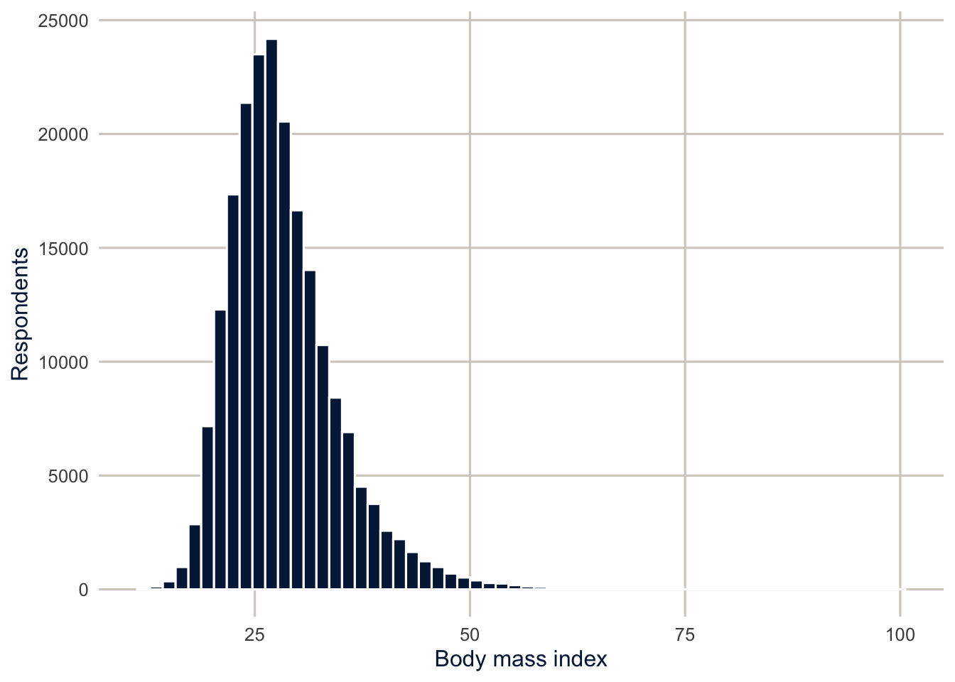
Box and whisker plots are a graphical version of Tukey’s five-number summary, and they’re a good way to compare a continuous variable across the levels of a categorical one. coord_flip() turns them on their side, and facet_wrap() makes a separate panel for each level of another variable, which lets you see whether a pattern is the same across groups.
brfss |>
  filter(!is.na(bmi), !is.na(sex)) |>
  ggplot(aes(x = agec, y = bmi)) +
  geom_boxplot(fill = utsa_cols("river_mist"), colour = utsa_cols("midnight"),
               outlier.alpha = 0.1) +
  facet_wrap(~sex) +
  coord_flip() +
  labs(x = "Age group", y = "Body mass index")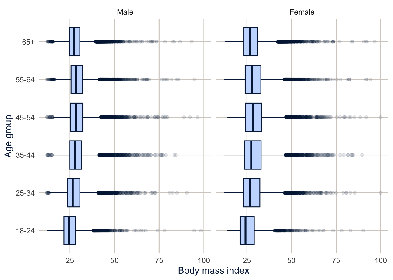
Median BMI rises through middle age and falls after 65 for both men and women, and the long right tail shows up as the cloud of outliers at every age. Is this everything R will do for describing data? No. Is this the only way to do it? Never. I’m constantly surprised by how many new functions I see students using in their own work, and it reminds me how much of the R ecosystem I have yet to explore.
Homework 1
Due: January 28, before class. Everyone in DEM 5283 and DEM 7283 does the same Homework 1. Exercises 6 and 7 use the survey you’re proposing in your survey data choice, which is due the same day (see the syllabus).
Purpose. Read a finished analysis closely, then set up the workflow you’ll use for every homework this semester.
What is provided. The course data section of this chapter, a short descriptive analysis of the BRFSS SMART file; the course repository; and R/get_mmsa.R.
What to turn in. Through Canvas, two links: your rendered homework on Posit Connect Cloud, and your GitHub repository.
A satisfactory answer renders from top to bottom without errors, answers each written question in complete sentences, and says whether each number describes the survey respondents or the population they represent.
1. Using The course data section of this chapter as your example, identify (a) the research question the section answers, (b) the unit represented by one row of the data, and (c) the population the data are intended to describe. Report one descriptive result from that section in a complete sentence. Then explain which files another reader would need to reproduce that result.
2. Create a folder for your homework this semester and open it in Positron with File > Open Folder. Follow steps 1 to 5 of the Git section to put it under version control and connect it to a new GitHub repository, and add data/ to its .gitignore. Run usethis::git_sitrep() and check that it reports no problems. Then change a file, commit it and push it, and check on GitHub that your commit arrived.
# YOUR CODE HERE3. Initialize renv in the project, install tidyverse and here, and take a snapshot. Show the output of renv::status().
# YOUR CODE HERE4. Copy R/get_mmsa.R into your project, read the 2024 MMSA data with it, and report the number of respondents and the sum of mmsawt for one metro area other than San Antonio. Use here() for every file path.
# YOUR CODE HEREOne solution for exercise 4
library(tidyverse)
library(here)
source(here("R", "get_mmsa.R"))

brfss <- get_mmsa(2024)

brfss |>
  filter(str_detect(mmsaname, "^Austin")) |>
  summarise(respondents = n(),
            adults_represented = sum(mmsawt))
5. For the metro area you chose in exercise 4, use dplyr to make a table of the number of respondents, the mean BMI and the percent who report fair or poor health (genhlth of 4 or 5) by sex and age group, and make one ggplot figure that shows how BMI differs by age. Remember that these are unweighted descriptions of the sample, and say so in a sentence.
# YOUR CODE HERE6. Download the survey you’re proposing for your survey data choice into your project’s data/ folder, and read it into R using here() for the file path. How many respondents and how many variables are in the file, and what does one row of the data represent?
# YOUR CODE HERE7. Using your survey’s documentation, identify the design variables: the weight, and either the strata and PSU (cluster) variables or the replicate weights. Report their names and what the documentation says each one is. Then sum the weight, and say what population that total represents.
# YOUR CODE HERE8. End your document with a chunk that runs sessionInfo(), render the document to a self-contained HTML file, then commit and push the .qmd file, the rendered HTML and renv.lock.
# YOUR CODE HERE9. Create a Posit Connect Cloud account and publish the rendered, self-contained HTML file from exercise 8 (not the .qmd) with whichever method you prefer. Open the link in a private browser window to check that it works, then commit the .posit/ folder or _publish.yml file that the publishing step created, and push.
Session information
sessionInfo()#> R version 4.6.2 (2026-10-29)
#> Platform: aarch64-apple-darwin23
#> Running under: macOS Tahoe 26.7.2
#>
#> Matrix products: default
#> BLAS: /Library/Frameworks/R.framework/Versions/4.6/Resources/lib/libRblas.0.dylib
#> LAPACK: /Library/Frameworks/R.framework/Versions/4.6/Resources/lib/libRlapack.dylib; LAPACK version 3.12.1
#>
#> locale:
#> [1] C.UTF-8/C.UTF-8/C.UTF-8/C/C.UTF-8/C.UTF-8
#>
#> time zone: America/Chicago
#> tzcode source: internal
#>
#> attached base packages:
#> [1] stats graphics grDevices datasets utils methods base
#>
#> other attached packages:
#> [1] sparkscolors_0.2.0 here_1.0.2 lubridate_1.9.5 forcats_1.0.1
#> [5] stringr_1.6.0 dplyr_1.2.1 purrr_1.2.2 readr_2.2.0
#> [9] tidyr_1.3.2 tibble_3.3.1 ggplot2_4.0.3 tidyverse_2.0.0
#>
#> loaded via a namespace (and not attached):
#> [1] gtable_0.3.6 jsonlite_2.0.0 compiler_4.6.2 renv_1.3.1
#> [5] tidyselect_1.2.1 scales_1.4.0 yaml_2.3.12 fastmap_1.2.0
#> [9] R6_2.6.1 labeling_0.4.3 generics_0.1.4 knitr_1.52
#> [13] htmlwidgets_1.6.4 rprojroot_2.1.1 tzdb_0.5.0 pillar_1.11.1
#> [17] RColorBrewer_1.1-3 rlang_1.3.0 utf8_1.2.6 stringi_1.8.9
#> [21] xfun_0.62 S7_0.2.2 otel_0.2.0 timechange_0.4.0
#> [25] cli_3.6.6 withr_3.0.3 magrittr_2.0.5 digest_0.6.39
#> [29] grid_4.6.2 hms_1.1.4 lifecycle_1.0.5 vctrs_0.7.3
#> [33] evaluate_1.0.5 glue_1.8.1 farver_2.1.2 rmarkdown_2.32
#> [37] tools_4.6.2 pkgconfig_2.0.3 htmltools_0.5.9Additional resources
- R for Data Science, 2nd edition (Wickham et al. 2023), free online. The place to go when the data management in these chapters moves faster than you’d like.
- Happy Git and GitHub for the useR, Jenny Bryan’s free guide to Git from R. Read it the first time Git does something you didn’t expect, which will be soon.
- The Quarto guide covers every option you’ll put in a document header, and plenty you won’t.
- Introduction to renv, the package vignette, explains what the lockfile records and what
restore()actually does.