library(tidyverse)
library(here)
library(survey)
library(marginaleffects)
library(modelsummary)
library(gtsummary)
library(sparkscolors)

source(here("R", "get_mmsa.R"))
source(here("R", "recode_mmsa.R"))Week 3: Binary Outcomes with Logit and Probit Models
Introduction
Most of the outcomes demographers care about aren’t continuous. Someone migrates or doesn’t, has a birth this year or doesn’t, dies before age 65 or doesn’t, reports poor health or doesn’t. Transitions (from employed to unemployed, from married to divorced) and thresholds (being obese, being in poverty) usually end up coded the same way, as a 1 or a 0. This week is about the workhorse models for those outcomes, the logit and the probit, fit to complex survey data.
The models themselves are not hard to fit. The hard part, and the part I want you to spend your time on, is saying what the results mean. Logit coefficients are changes in log-odds, which nobody thinks in. Odds ratios are better, but they are routinely misread as risk ratios. So most of this document is about turning model output into predicted probabilities and average marginal effects, the quantities you should report in your papers (Mood 2010; Breen et al. 2018).
NoteThis week at a glance
The question. How much more likely are adults with less education, or Hispanic adults, to report fair or poor health than other adults of the same age and sex?
By the end of this week you should be able to
- convert between a probability, odds, log-odds and an odds ratio, by hand;
- fit a survey-weighted logit model and interpret an odds ratio, naming the comparison group;
- report an adjusted difference in probabilities in percentage points, and describe it as an association, not an effect.
Before you begin. You’ll use the survey design object from week 2, svyglm() from the week 2 regression section, and the map() pattern from week 2. From your first course, you need linear regression and the idea of a reference category for a categorical predictor.
Required and optional. The probit and the other links are an alternative way to write the same kind of model; the section on them is optional on a first reading. Everything else is required.
Setup
marginaleffects does the post-estimation work. It handles predicted probabilities, comparisons and marginal effects for almost any model in R, including svyglm().
Generalized linear models for binary outcomes
From the linear model to the GLM
Up to now you’ve mostly relied on linear models that assume Normal errors. Strictly, that’s an assumption about the conditional distribution of the outcome: for people with the same values of the predictors, the outcomes are spread out Normally around the regression line. The raw outcome itself doesn’t have to look Normal. A broader class, generalized linear models or GLMs (Nelder and Wedderburn 1972), allows regression for outcomes that aren’t Normal. Every GLM has three parts: a probability distribution suited to the outcome, a linear predictor made of the coefficients and covariates, and a link function that connects the mean of the distribution to the linear predictor. The linear model is a GLM, too. Its mean is \(\mu\), and the linear predictor is connected to it directly:
\[ g(\mu) = g(E(Y)) = \beta_0 + \beta_1 x_1, \qquad g(\mu) = \mu \]
That’s the identity link: no transformation at all. It works for the Normal because the Normal can take any value from \(-\infty\) to \(\infty\), so a straight line can’t wander off the scale of the data. Other distributions have narrower ranges, and their links transform the mean so the linear predictor stays on the right scale.
For a binary outcome, the distribution is the binomial, which you’ve probably met in a basic statistics course (remember the coin flips?). It gets used in two ways. When each person has a single “trial,” with an outcome of 1 or 0, it’s called the Bernoulli distribution, and that’s the logistic regression you’ve probably seen before. When we have \(y\) events out of \(n\) trials, which is the basic makeup of a demographic rate (deaths out of people at risk, low birth weight births out of all births), we have what I call the count-based binomial. Either way the mean is a probability, \(\pi\), and the model says how that probability depends on the predictors. For a single person \(i\), the expected value of a 0/1 outcome is the probability that it’s 1:
\[ E(Y_i \mid \mathbf{x}_i) = \Pr(Y_i = 1 \mid \mathbf{x}_i) = \pi_i = \text{some function of } \mathbf{x}_i \]
Read the vertical bar as “given”: the probability for someone with predictor values \(\mathbf{x}_i\). For grouped data, with \(Y_j\) events out of \(n_j\) trials in group \(j\), the observed proportion \(Y_j / n_j\) is our estimate of \(\pi_j\), but it isn’t the same thing. The probability is a property of the population (or the model), and the observed proportion bounces around it from sample to sample.
This week is about the Bernoulli case, with individual survey respondents. We’ll use the count-based binomial for rates in places in week 6.
Why not the linear model?
If \(y_i\) is 1 or 0, its mean is a probability, \(\pi_i = P(y_i = 1)\), and its variance is \(\pi_i(1 - \pi_i)\). A linear model for \(\pi_i\) (the linear probability model) has two problems. The variance depends on the mean, so the errors can’t be homoskedastic, and nothing stops the fitted values from going below 0 or above 1. The linear probability model has defenders, mostly in economics, and I’ll come back to it at the end, because its coefficients are often close to the average marginal effects from a logit. But for most demographic work we want a model that respects the bounds.
Link functions
A generalized linear model (GLM) keeps the linear predictor, \(\eta_i = \mathbf{x}_i'\boldsymbol\beta\), and connects it to the mean through a link function \(g()\), so that \(g(\pi_i) = \eta_i\). The link stretches the interval from 0 to 1 onto the whole real line. The logit link is the log of the odds:
\[ \text{logit}(\pi_i) = \log\left(\frac{\pi_i}{1 - \pi_i}\right) = \mathbf{x}_i'\boldsymbol\beta \quad\Longleftrightarrow\quad \pi_i = \frac{1}{1 + \exp(-\mathbf{x}_i'\boldsymbol\beta)} \]
It’s worth walking through that one step at a time. The odds of an event are the probability it happens divided by the probability it doesn’t, \(\pi / (1 - \pi)\). A probability is stuck between 0 and 1, but the odds run from 0 to \(\infty\), and taking the log of the odds stretches that onto the whole real line, from \(-\infty\) to \(\infty\). Now a linear function of the covariates can’t go out of bounds, and we can write the model as \(\text{logit}(\pi) = \beta_0 + \beta_1 x_1\) without worrying about the boundary problem.
Here’s one number taken all the way through, because these scales are easy to mix up:
| Scale | Value | How you get it |
|---|---|---|
| Probability | 0.20 | 20 people in 100 |
| Odds | 0.25 | \(0.20 / (1 - 0.20) = 0.20 / 0.80\) |
| Log-odds (logit) | \(-1.39\) | \(\log(0.25)\) |
| Odds doubled | 0.50 | \(2 \times 0.25\) |
| Back to a probability | 0.333 | \(\text{odds} / (1 + \text{odds}) = 0.50 / 1.50\) |
Doubling the odds took the probability from 0.20 to 0.333, not to 0.40. An odds ratio of 2 doesn’t mean the probability doubles, and we’ll come back to that at the end of the chapter.
Probit and other links (optional on a first reading)
The logit is the model we’ll use most, and you can skip this section the first time through. The probit link is the inverse of the standard normal cumulative distribution function, \(\Phi^{-1}(\pi_i) = \mathbf{x}_i'\boldsymbol\beta\), so \(\pi_i = \Phi(\mathbf{x}_i'\boldsymbol\beta)\). A third link, the complementary log-log, \(\log(-\log(1 - \pi_i)) = \mathbf{x}_i'\boldsymbol\beta\), is asymmetric, and it comes up mostly when the binary outcome is really whether an event happened in an interval of time, which is why you’ll see it again in your event history course.
Both models can also be written as models for a latent propensity \(y_i^* = \mathbf{x}_i'\boldsymbol\beta + \varepsilon_i\), where we only see \(y_i = 1\) when \(y_i^* > 0\). The logit assumes \(\varepsilon\) has a logistic distribution (variance \(\pi^2/3\)), and the probit assumes a standard normal (variance 1). That’s the whole difference between them, and it’s why logit coefficients are about 1.6 to 1.8 times the size of probit coefficients for the same data. It’s also the source of the nested model problem we’ll take on in week 4.
tibble(eta = seq(-6, 6, by = 0.05)) |>
  mutate(Logit = plogis(eta),
         Probit = pnorm(eta / 1.7)) |>
  pivot_longer(-eta, names_to = "link", values_to = "probability") |>
  ggplot(aes(x = eta, y = probability, colour = link, linetype = link)) +
  geom_line(linewidth = 1.2) +
  scale_colour_utsa(palette = "primary") +
  labs(x = "Linear predictor", y = "Probability", colour = NULL, linetype = NULL)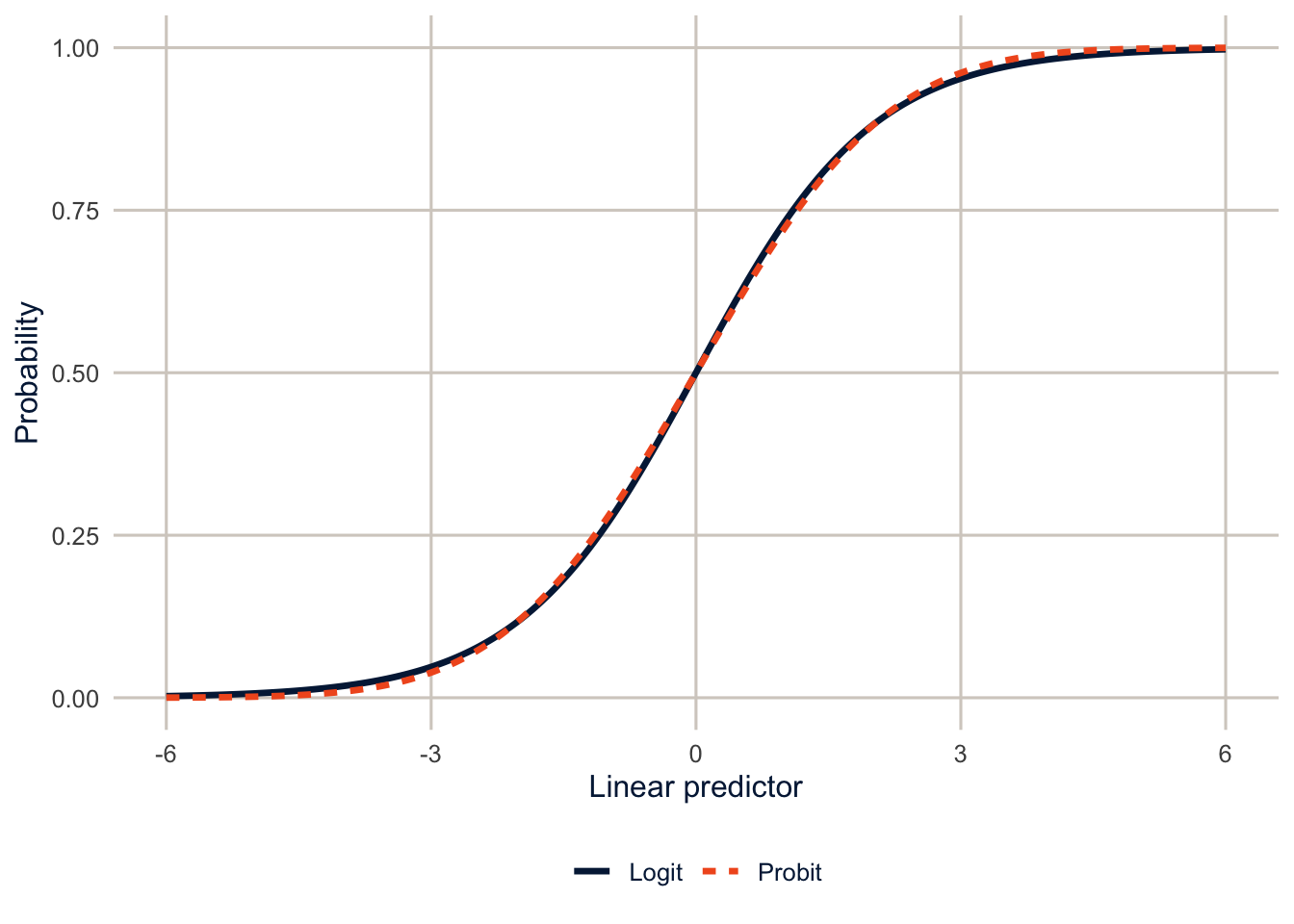
Odds and odds ratios
Because we modeled the log of the odds, the coefficients are on the log-odds scale, not a linear one. We can read their signs directly (a positive \(\beta\) raises the odds of \(y = 1\), a negative one lowers them), but the usual interpretation is the odds ratio, which you get by exponentiating the coefficient. The percent change in the odds for a one-unit change in \(x_1\) is
\[ \%\Delta \text{ odds} = 100 \times \left(\exp(\beta_1) - 1\right) \]
So a \(\beta_1\) of 0.025 gives \(\exp(0.025) = 1.025\), and a one-unit increase in \(x_1\) raises the odds of \(y\) by 2.5%. If \(\beta_1 = 0.4\), then \(\exp(0.4) = 1.49\), a 49% increase in the odds. A negative coefficient works the same way: \(\beta_1 = -0.15\) gives \(\exp(-0.15) - 1 = -0.14\), a 14% decrease. Odds ratios are constant across the range of \(x\), which is convenient, but odds are not probabilities, and that difference will come back below.
An odds ratio is always a comparison between two groups, so always say what’s being compared with what. For a categorical predictor, the comparison is with the reference category, the level left out of the model (here, the first level of each factor). “Hispanic adults have 1.5 times the odds” is incomplete; “Hispanic adults have 1.5 times the odds of non-Hispanic White adults with the same education, age and sex” is a complete sentence.
The data and some descriptive work
The outcome is fair or poor self-rated health in the 2024 BRFSS SMART MMSA file. Self-rated health is one of the best single predictors of mortality we have, and it’s asked in almost every health survey, which makes it a good teaching outcome. recode_mmsa() makes the variables from week 2.
brfss <- get_mmsa(2024) |> recode_mmsa()
des <- svydesign(ids = ~1, strata = ~ststr, weights = ~mmsawt, data = brfss)
Before any model, look at the outcome by the main predictors. svyciprop() gives design-based confidence intervals for proportions.
desc <- c("educ", "race_eth") |>
  set_names() |>
  map(\(v) {
    res <- svyby(~badhealth, reformulate(v), design = des, FUN = svyciprop,
                 vartype = "ci", na.rm = TRUE)
    tibble(group = as.character(res[[v]]), estimate = coef(res),
           ci_l = res$ci_l, ci_u = res$ci_u)
  }) |>
  list_rbind(names_to = "variable") |>
  mutate(variable = if_else(variable == "educ", "Education", "Race and ethnicity"),
         group = fct_inorder(group))

svychisq(~badhealth + educ, design = des)
#>
#> Pearson's X^2: Rao & Scott adjustment
#>
#> data: svychisq(~badhealth + educ, design = des)
#> F = 775.81, ndf = 2.7835e+00, ddf = 6.3863e+05, p-value < 2.2e-16
NoteCode explanation: building a formula from text
recode_mmsa() (in R/recode_mmsa.R) does the week 2 recodes in one step, so every chapter starts from the same variables.
The descriptive pipe runs the same svyby() for two variables, using the map() pattern from week 2. Two new pieces:
set_names()names each element ofc("educ", "race_eth")with its own value, so the results come back labelededucandrace_eth, andlist_rbind(names_to = "variable")can use those names.reformulate(v)turns the text"educ"into the formula~educ.svyby()wants a formula, and inside the functionvis just text, so this converts it.res[[v]]then pulls out the column whose name is stored inv.
desc |>
  ggplot(aes(x = estimate, y = fct_rev(group))) +
  geom_pointrange(aes(xmin = ci_l, xmax = ci_u), colour = utsa_cols("midnight")) +
  facet_wrap(~variable, scales = "free_y", ncol = 1) +
  scale_x_continuous(labels = scales::label_percent(), limits = c(0, NA)) +
  labs(x = "Fair or poor health", y = NULL)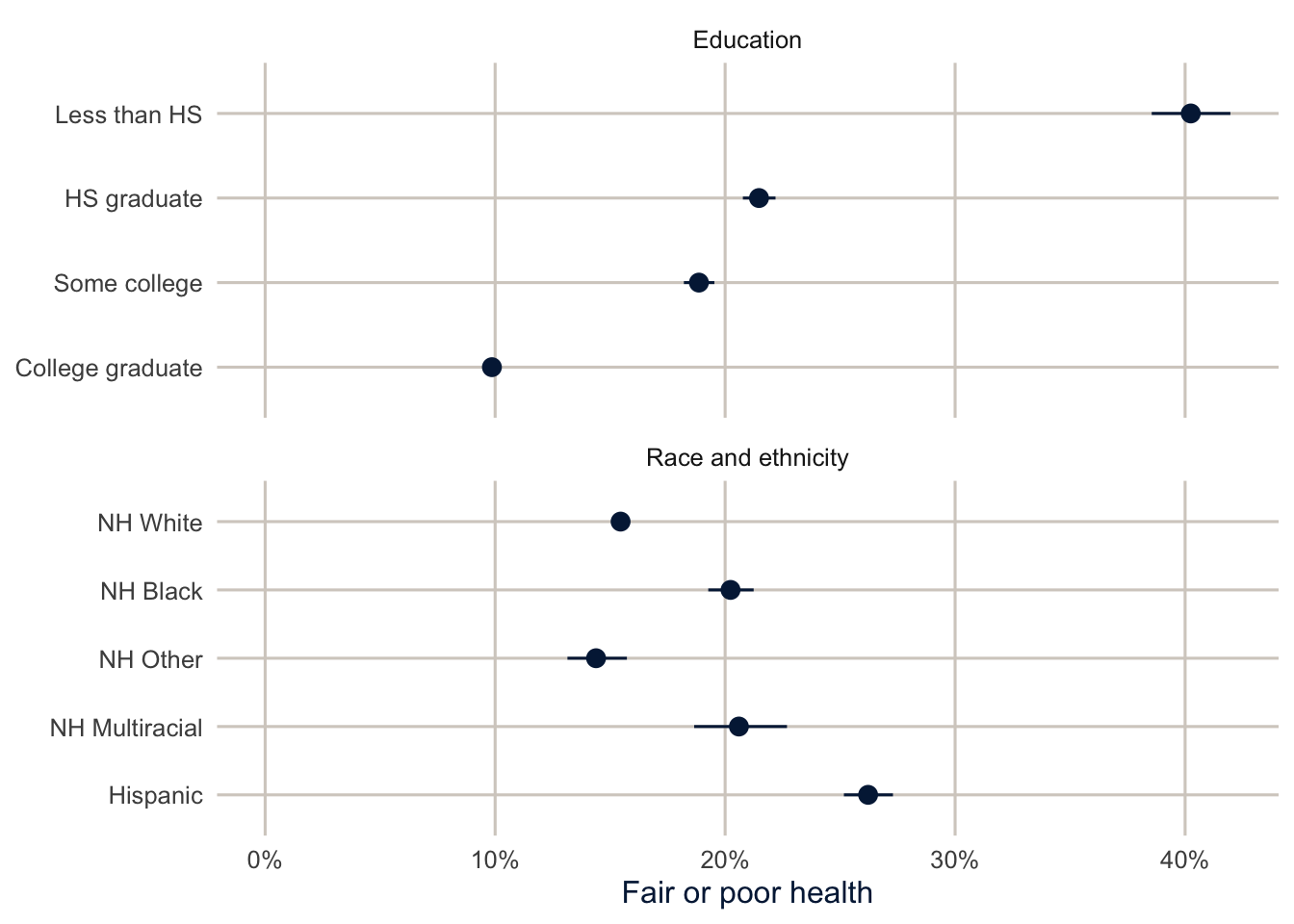
The education gradient is steep, and Hispanic adults report fair or poor health at a higher rate than any other group. Part of that is education, and part may be about how the question works across languages and cultures (a long-standing debate in the Hispanic health literature). The model below starts to separate the first part out.
Before the model, though, it’s worth looking at the two variables together. svyby() with two grouping variables gives the prevalence for every combination of race and ethnicity and education.
race_educ <- svyby(~badhealth, ~race_eth + educ, design = des, FUN = svymean,
                   na.rm = TRUE)

race_educ |>
  as_tibble() |>
  mutate(ci_l = badhealth - 1.96 * se, ci_u = badhealth + 1.96 * se) |>
  ggplot(aes(x = educ, y = badhealth, colour = race_eth, shape = race_eth,
             group = race_eth)) +
  geom_line(position = position_dodge(width = 0.4)) +
  geom_pointrange(aes(ymin = ci_l, ymax = ci_u), position = position_dodge(width = 0.4)) +
  scale_colour_utsa() +
  scale_y_continuous(labels = scales::label_percent()) +
  labs(x = NULL, y = "Fair or poor health", colour = NULL, shape = NULL)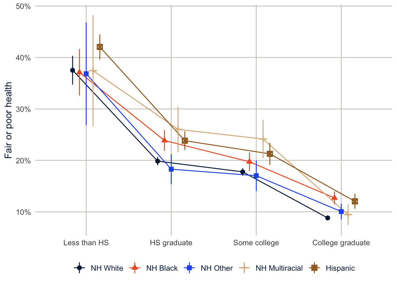
The education gradient shows up in every group, and within each level of education the racial and ethnic differences are much smaller than they were overall. The overall Hispanic-White gap is 10.8 percentage points, and within education groups it runs from 3.2 to 4.5. That’s the descriptive version of what the model will tell us: some, but not all, of the Hispanic disadvantage is about education.
Fitting logit and probit models
Logit and probit models for survey data are just svyglm() with a binomial family. I use quasibinomial(), which gives exactly the same estimates as binomial() but doesn’t warn about non-integer weights.
fit_logit <- svyglm(badhealth ~ race_eth + educ + agec + female,
                    design = des, family = quasibinomial())

fit_probit <- svyglm(badhealth ~ race_eth + educ + agec + female,
                     design = des, family = quasibinomial(link = "probit"))

summary(fit_logit)
#>
#> Call:
#> svyglm(formula = badhealth ~ race_eth + educ + agec + female,
#> design = des, family = quasibinomial())
#>
#> Survey design:
#> svydesign(ids = ~1, strata = ~ststr, weights = ~mmsawt, data = brfss)
#>
#> Coefficients:
#> Estimate Std. Error t value Pr(>|t|)
#> (Intercept) -1.41064 0.06110 -23.087 < 2e-16 ***
#> race_ethNH Black 0.26653 0.03571 7.464 8.39e-14 ***
#> race_ethNH Other 0.17266 0.05792 2.981 0.00287 **
#> race_ethNH Multiracial 0.46511 0.06606 7.041 1.91e-12 ***
#> race_ethHispanic 0.42880 0.03609 11.883 < 2e-16 ***
#> educHS graduate -0.72464 0.04490 -16.139 < 2e-16 ***
#> educSome college -0.94626 0.04620 -20.480 < 2e-16 ***
#> educCollege graduate -1.68825 0.04551 -37.098 < 2e-16 ***
#> agec25-34 0.27387 0.05648 4.849 1.24e-06 ***
#> agec35-44 0.44910 0.05493 8.176 2.95e-16 ***
#> agec45-54 0.77399 0.05405 14.320 < 2e-16 ***
#> agec55-64 0.97025 0.05155 18.823 < 2e-16 ***
#> agec65+ 1.07579 0.04921 21.860 < 2e-16 ***
#> female 0.09881 0.02519 3.922 8.78e-05 ***
#> ---
#> Signif. codes: 0 '***' 0.001 '**' 0.01 '*' 0.05 '.' 0.1 ' ' 1
#>
#> (Dispersion parameter for quasibinomial family taken to be 1.002631)
#>
#> Number of Fisher Scoring iterations: 4
NoteCode explanation: logit and probit models with
svyglm()
svyglm() is the same function you used for BMI in week 2. The family argument says what kind of outcome it is. quasibinomial() uses the logit link by default, and quasibinomial(link = "probit") switches to the probit. summary() prints the coefficients, their standard errors, \(t\) statistics and p-values, all on the log-odds scale for the logit.
The coefficients are on the log-odds scale. Positive values mean higher odds of fair or poor health, so everything here goes in the direction the descriptive figures suggested. To test whether a whole set of dummies matters, use a design-based Wald test (likelihood ratio tests aren’t valid with survey weights):
regTermTest(fit_logit, ~race_eth, method = "Wald")#> Wald test for race_eth
#> in svyglm(formula = badhealth ~ race_eth + educ + agec + female,
#> design = des, family = quasibinomial())
#> F = 48.73079 on 4 and 223010 df: p= < 2.22e-16regTermTest() tests whether all the coefficients for a variable (here, the four race and ethnicity dummies) are zero at once. The second argument names the variable with a formula. Read its p-value like any other: a small one says race and ethnicity, as a whole, is associated with the outcome after adjusting for the rest of the model.
Here are the odds ratios next to the probit coefficients:
modelsummary(list("Logit (odds ratios)" = fit_logit, "Probit" = fit_probit),
             exponentiate = c(TRUE, FALSE),
             fmt = 3,
             coef_omit = "Intercept",
             coef_rename = \(x) str_remove_all(x, "race_eth|educ|agec"),
             gof_map = "nobs",
title = "Models for fair or poor self-rated health")| Logit (odds ratios) | Probit | |
|---|---|---|
| NH Black | 1.305 | 0.150 |
| (0.047) | (0.020) | |
| NH Other | 1.188 | 0.097 |
| (0.069) | (0.032) | |
| NH Multiracial | 1.592 | 0.253 |
| (0.105) | (0.037) | |
| Hispanic | 1.535 | 0.241 |
| (0.055) | (0.021) | |
| HS graduate | 0.485 | -0.441 |
| (0.022) | (0.027) | |
| Some college | 0.388 | -0.564 |
| (0.018) | (0.028) | |
| College graduate | 0.185 | -0.968 |
| (0.008) | (0.027) | |
| 25-34 | 1.315 | 0.157 |
| (0.074) | (0.030) | |
| 35-44 | 1.567 | 0.250 |
| (0.086) | (0.029) | |
| 45-54 | 2.168 | 0.425 |
| (0.117) | (0.029) | |
| 55-64 | 2.639 | 0.536 |
| (0.136) | (0.028) | |
| 65+ | 2.932 | 0.602 |
| (0.144) | (0.026) | |
| female | 1.104 | 0.057 |
| (0.028) | (0.014) | |
| Num.Obs. | 224220 | 224220 |
In modelsummary(), exponentiate = c(TRUE, FALSE) exponentiates the first model’s coefficients (turning log-odds into odds ratios) and leaves the second’s alone, and coef_omit = "Intercept" drops the intercept row.
College graduates have 0.18 times the odds of fair or poor health of adults without a high school diploma, so their odds are 82% lower. Hispanic adults have 1.54 times the odds of non-Hispanic White adults with the same education, age and sex. The ratio of logit to probit coefficients runs from about 1.7 to 1.8 for most terms, so the two models say the same thing in different units. Both show higher chances of fair or poor health for every group compared with non-Hispanic White adults (the reference group), most of all for Hispanic and multiracial adults, a steady decline with each step up in education compared with not finishing high school, and a steady rise with age compared with adults under 25. If you do report odds ratios, report them with confidence intervals. tbl_regression() from gtsummary exponentiates the coefficients, computes design-based intervals, and lays out the reference groups clearly:
tbl_regression(fit_logit, exponentiate = TRUE,
               label = list(race_eth ~ "Race and ethnicity", educ ~ "Education",
                            agec ~ "Age group", female ~ "Female")) |>
bold_labels()| Characteristic | OR | 95% CI | p-value |
|---|---|---|---|
| Race and ethnicity | |||
| NH White | — | — | |
| NH Black | 1.31 | 1.22, 1.40 | <0.001 |
| NH Other | 1.19 | 1.06, 1.33 | 0.003 |
| NH Multiracial | 1.59 | 1.40, 1.81 | <0.001 |
| Hispanic | 1.54 | 1.43, 1.65 | <0.001 |
| Education | |||
| Less than HS | — | — | |
| HS graduate | 0.48 | 0.44, 0.53 | <0.001 |
| Some college | 0.39 | 0.35, 0.42 | <0.001 |
| College graduate | 0.18 | 0.17, 0.20 | <0.001 |
| Age group | |||
| 18-24 | — | — | |
| 25-34 | 1.32 | 1.18, 1.47 | <0.001 |
| 35-44 | 1.57 | 1.41, 1.75 | <0.001 |
| 45-54 | 2.17 | 1.95, 2.41 | <0.001 |
| 55-64 | 2.64 | 2.39, 2.92 | <0.001 |
| 65+ | 2.93 | 2.66, 3.23 | <0.001 |
| Female | 1.10 | 1.05, 1.16 | <0.001 |
| Abbreviations: CI = Confidence Interval, OR = Odds Ratio | |||
tbl_regression() is the gtsummary table for a fitted model, the partner of tbl_svysummary() from week 2. exponentiate = TRUE shows odds ratios, and the reference category of each variable gets its own row, marked with a dash, so a reader can see what each odds ratio compares against.
A picture is often easier to digest. On the odds ratio scale, an interval that crosses 1 means the effect isn’t statistically different from zero. I put the axis on a log scale, because an odds ratio of 0.5 is as far from 1 as an odds ratio of 2.
broom::tidy(fit_logit, conf.int = TRUE, exponentiate = TRUE) |>
  filter(term != "(Intercept)") |>
  mutate(term = str_remove_all(term, "race_eth|educ|agec"),
         term = fct_inorder(term)) |>
  ggplot(aes(x = estimate, y = fct_rev(term))) +
  geom_vline(xintercept = 1, colour = utsa_cols("smoke"), linewidth = 1) +
  geom_pointrange(aes(xmin = conf.low, xmax = conf.high), colour = utsa_cols("midnight")) +
  scale_x_log10() +
  labs(x = "Odds ratio", y = NULL)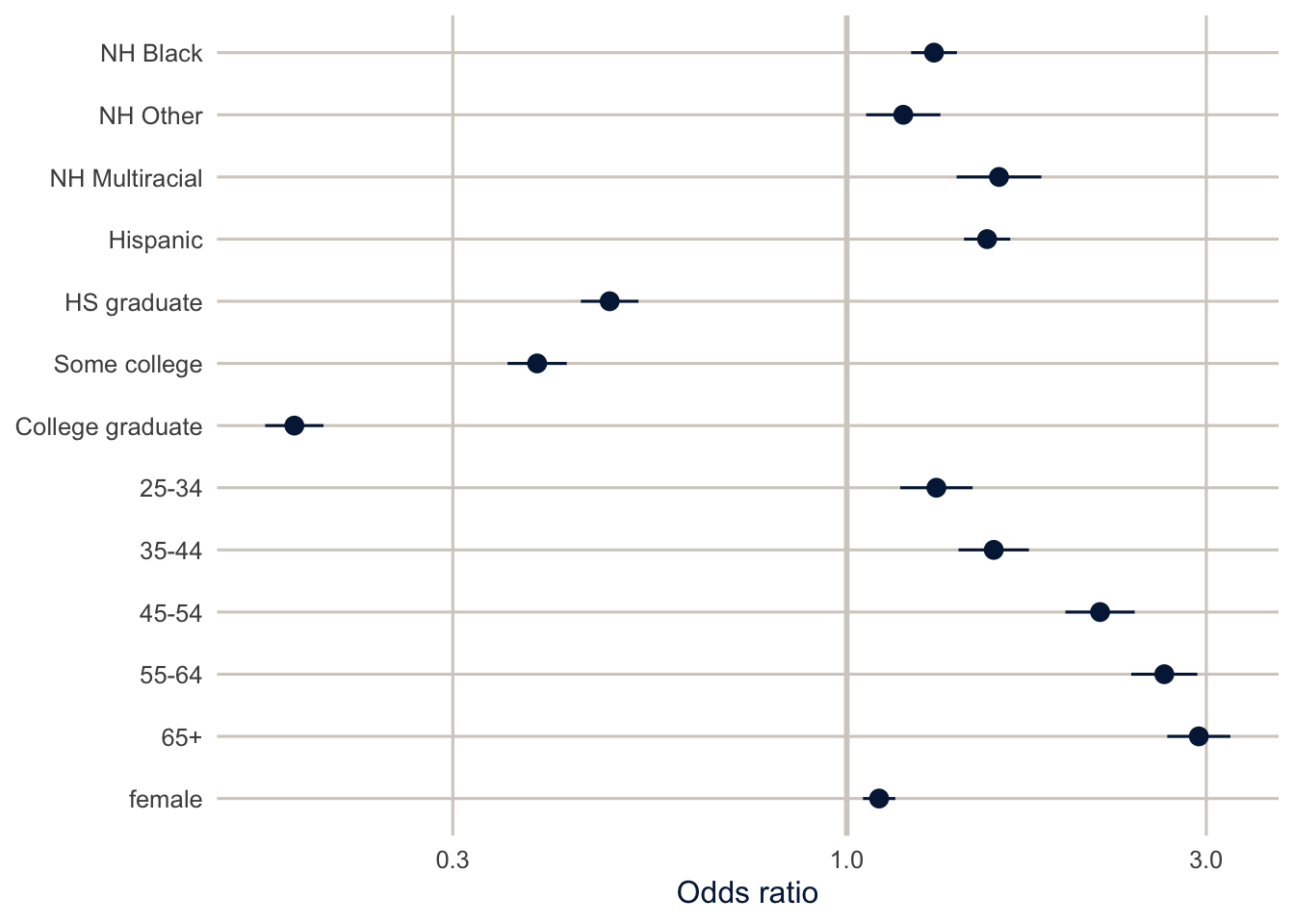
From coefficients to probabilities
Predicted probabilities for particular people
As I often say, I like to talk about interesting cases. To do that, we need the fitted probability for a particular kind of person, and getting it just means “solving the equation” for the model at the values of \(x\) that describe that person. For a non-Hispanic White woman age 45 to 54 with a college degree, everything but the intercept, the college dummy, the age dummy and the female dummy is zero, so
\[ \Pr(\text{fair/poor health}) = \frac{1}{1 + \exp\left[-(\beta_0 + \beta_{\text{college}} + \beta_{45\text{-}54} + \beta_{\text{female}})\right]} \]
Here it is by hand:
b <- coef(fit_logit)
eta <- b[["(Intercept)"]] + b[["educCollege graduate"]] + b[["agec45-54"]] + b[["female"]]
plogis(eta)   # plogis() is the inverse logit, 1 / (1 + exp(-eta))
#> [1] 0.09743142
NoteCode explanation: a prediction by hand
coef(fit_logit) returns the coefficients as a named vector, and b[["educCollege graduate"]] pulls out one by its name (the variable name followed by the category). Adding the intercept and the three coefficients that apply to this woman gives her linear predictor, eta, on the log-odds scale. plogis() converts log-odds to a probability, which is the right-hand side of the logit equation above.
Doing that for many kinds of people gets tedious, and it doesn’t give you a confidence interval. So what’s the predicted probability of fair or poor health for a 45-to-54-year-old woman, by race and ethnicity and education? datagrid() builds the “people,” and predictions() computes their probabilities with confidence intervals.
cases <- predictions(fit_logit,
                     newdata = datagrid(race_eth = c("NH White", "NH Black", "Hispanic"),
                                        educ = c("HS graduate", "College graduate"),
                                        agec = "45-54",
                                        female = 1))

cases |>
  as_tibble() |>
  select(race_eth, educ, estimate, conf.low, conf.high) |>
knitr::kable(digits = 3)| race_eth | educ | estimate | conf.low | conf.high |
|---|---|---|---|---|
| NH White | HS graduate | 0.221 | 0.207 | 0.234 |
| NH White | College graduate | 0.097 | 0.091 | 0.104 |
| NH Black | HS graduate | 0.270 | 0.251 | 0.289 |
| NH Black | College graduate | 0.124 | 0.113 | 0.134 |
| Hispanic | HS graduate | 0.303 | 0.283 | 0.323 |
| Hispanic | College graduate | 0.142 | 0.130 | 0.154 |
NoteCode explanation:
datagrid() and predictions()
datagrid() builds a small data frame of made-up people. Each argument gives the values of one variable, and datagrid() makes every combination: here 3 race and ethnicity groups times 2 education levels, all 45 to 54 and female, for 6 rows. predictions(model, newdata = ...) computes each row’s predicted probability with a confidence interval. The result has one row per made-up person, with the prediction in estimate and the interval in conf.low and conf.high.
For a Hispanic woman in her late 40s with a high school diploma, the model predicts a 30.3% chance of reporting fair or poor health. For a non-Hispanic White woman with a college degree, it’s 9.7%, the same number we got by hand. Sentences like these are far easier for a reader to hold on to than “the odds ratio is 0.18.”
Average predictions
Choosing interesting cases is a judgment call, and the results depend on what you hold the other variables at. Average predictions avoid the choice. For each level of education, set everyone’s education to that level, keep everything else as observed, predict, and average over the sample with the survey weights.
avg_predictions(fit_logit, variables = "educ", wts = "(weights)")#>
#> educ Estimate Std. Error z Pr(>|z|) S 2.5 % 97.5 %
#> Less than HS 0.367 0.00867 42.3 <0.001 Inf 0.3499 0.384
#> HS graduate 0.223 0.00372 59.9 <0.001 Inf 0.2156 0.230
#> Some college 0.188 0.00350 53.6 <0.001 Inf 0.1808 0.194
#> College graduate 0.100 0.00197 51.0 <0.001 Inf 0.0963 0.104
#>
#> Type: responseThis is standardization, the same idea as an age-standardized rate. Each average prediction answers: “according to the model, what share of adults would report fair or poor health if the population had its actual mix of race and ethnicity, age and sex, but everyone was in this education group?” Because every education group is averaged over the same population, differences between them aren’t due to differences in age, sex or race and ethnicity.
Be careful with the “if everyone was in this education group” part, though. It describes a comparison the model makes, not what would happen if we actually changed people’s education. That’s a causal claim, and it needs assumptions we haven’t made yet (about everything else that differs between people with more and less education). Week 14 is about those assumptions. Until then, describe these as adjusted associations.
In avg_predictions(), variables = "educ" says which variable to set to each of its levels in turn, and wts = "(weights)" makes the averaging use the survey weights. svyglm() stores the weights under the name (weights), parentheses included, which is why it’s written that way.
Average marginal effects
The average marginal effect (AME) of a categorical predictor is the difference between two of these average predictions. For a continuous predictor, it’s the average of the slope of the probability curve. Either way, it’s on the probability scale.
ame_logit <- avg_comparisons(fit_logit, variables = c("race_eth", "educ"),
                             wts = "(weights)")
ame_logit
#>
#> Term Contrast Estimate Std. Error z Pr(>|z|)
#> educ College graduate - Less than HS -0.2667 0.00903 -29.55 <0.001
#> educ HS graduate - Less than HS -0.1441 0.00955 -15.09 <0.001
#> educ Some college - Less than HS -0.1793 0.00954 -18.79 <0.001
#> race_eth Hispanic - NH White 0.0619 0.00559 11.07 <0.001
#> race_eth NH Black - NH White 0.0368 0.00518 7.10 <0.001
#> race_eth NH Multiracial - NH White 0.0678 0.01071 6.33 <0.001
#> race_eth NH Other - NH White 0.0232 0.00812 2.86 0.0043
#> S 2.5 % 97.5 %
#> 634.9 -0.28441 -0.2490
#> 168.4 -0.16277 -0.1253
#> 259.4 -0.19800 -0.1606
#> 92.2 0.05093 0.0728
#> 39.6 0.02661 0.0469
#> 31.9 0.04680 0.0888
#> 7.9 0.00726 0.0391
#>
#> Type: responseavg_comparisons() computes the differences between the average predictions for each level of a variable and its reference level, with design-based confidence intervals. Each row of the output is one comparison: the contrast column says which two groups, and estimate is the difference in probability (multiply by 100 for percentage points).
A college degree, compared with not finishing high school, is associated with a 26.7 percentage point lower probability of fair or poor health, averaged over the population. Being Hispanic rather than non-Hispanic White is associated with a probability 6.2 points higher.
TipReading the result: a right and a wrong interpretation
Right: “Adults with a college degree are 26.7 percentage points less likely to report fair or poor health than adults who didn’t finish high school, comparing people with the same race and ethnicity, age and sex.”
Wrong: “Getting a college degree lowers a person’s chance of fair or poor health by 26.7 percentage points.” That’s a causal claim about what happens to someone who gets more education. The model compares different people who already differ in education, and plenty else about them (income, childhood health, where they grew up) differs too. Say “is associated with” or “are less likely,” and save “lowers” for when you’ve made the case for a cause.
Notice the units, too. A percentage point difference subtracts one percentage from another: from 30% to 20% is 10 percentage points. A percent (relative) change divides: from 30% to 20% is a 33% decrease. Both are correct descriptions of the same change, and mixing them up makes effects sound bigger or smaller than they are. AMEs are percentage point differences; risk ratios (below) are relative.
Note
You’ll also see marginal effects at the mean (MEMs), which compute the slope for a single made-up person with every variable at its mean. With categorical predictors, that person is a fraction Hispanic and a fraction college graduate, which describes nobody. AMEs average over real people instead, and they’re the better default (Mood 2010). If you want effects for a specific kind of person, use datagrid() and say so.
Logit, probit, or a linear probability model?
Here are the AMEs for education and race from the logit, the probit, and a linear probability model (which is just svyglm() with a Gaussian family, so its coefficients are differences in probability).
fit_lpm <- svyglm(badhealth ~ race_eth + educ + agec + female,
                  design = des, family = gaussian())

ame_all <- list(Logit = fit_logit, Probit = fit_probit, LPM = fit_lpm) |>
  map(\(m) avg_comparisons(m, variables = c("race_eth", "educ"), wts = "(weights)")) |>
  map(as_tibble) |>
  list_rbind(names_to = "model") |>
  mutate(model = fct_inorder(model),
         contrast = str_remove(contrast, " - .*$"),
         label = paste0(if_else(term == "educ", "Educ: ", "Race: "), contrast),
         label = factor(label, levels = c(paste0("Educ: ", levels(brfss$educ)[-1]),
                                          paste0("Race: ", levels(brfss$race_eth)[-1]))))
NoteCode explanation: stacking the three models’ AMEs
This is the map() pattern from week 2, run twice: once to compute the AMEs for each model, and once (map(as_tibble)) to turn each result into a data frame before stacking. In the mutate(), str_remove(contrast, " - .*$") deletes everything from ” - ” to the end of the contrast label (.*$ means “anything, up to the end”), so “College graduate - Less than HS” becomes “College graduate”. paste0() glues a prefix onto each label, and factor(..., levels = ...) puts the labels in the same order as the categories. levels(brfss$educ)[-1] is every education level except the first; [-1] drops the first element, the reference group, which has no AME of its own.
ame_all |>
  ggplot(aes(x = estimate, y = fct_rev(label), colour = model, shape = model)) +
  geom_vline(xintercept = 0, colour = utsa_cols("smoke")) +
  geom_pointrange(aes(xmin = conf.low, xmax = conf.high),
                  position = position_dodge(width = 0.6)) +
  scale_colour_utsa() +
  scale_x_continuous(labels = scales::label_number(scale = 100, suffix = " pts")) +
  labs(x = "Average marginal effect", y = NULL, colour = NULL, shape = NULL)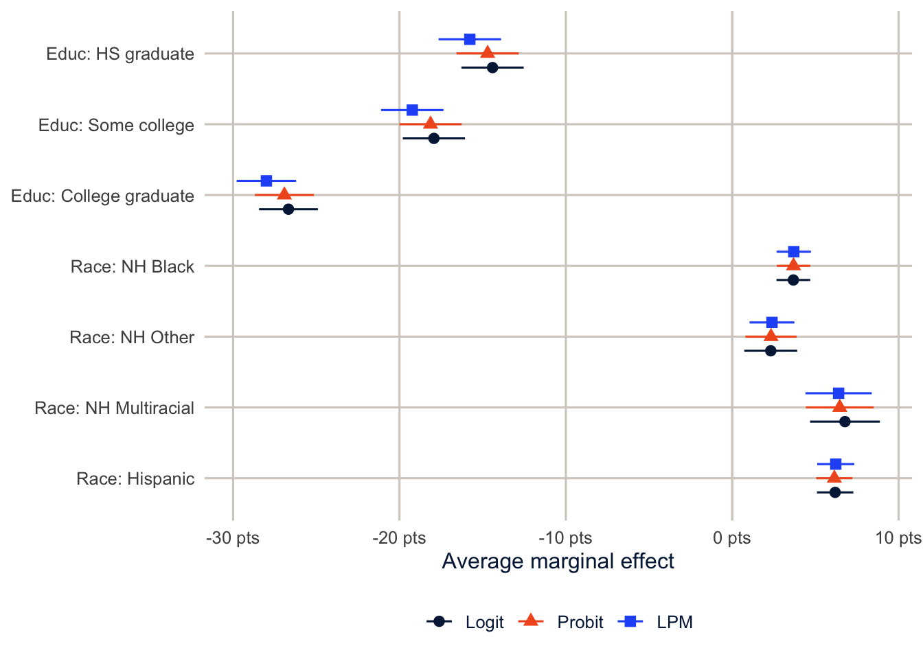
The three models agree closely on the probability scale, which is the usual result when the outcome isn’t too rare and the predictors are mostly categorical. That’s the case for the linear probability model: easy to explain, and often the same answer. The case against it is that its individual predictions can fall outside 0 and 1, and its effects are forced to be the same for everyone, which matters when you care about how an effect differs across people with different baseline risks. My advice is to fit a logit or probit, report AMEs, and check that a linear probability model tells the same story.
lpm_fitted <- predict(fit_lpm)
range(lpm_fitted)
#> [1] -0.01930623 0.49245739sum(lpm_fitted < 0)#> [1] 2033predict() returns each respondent’s fitted value from the model, range() gives the smallest and largest, and sum(lpm_fitted < 0) counts the negative ones (TRUE counts as 1 and FALSE as 0).
Here 2033 respondents get negative predicted probabilities. That’s harmless for the AMEs, but it’s a reminder that the linear probability model isn’t a model of individual probabilities.
Odds ratios are not risk ratios
One last thing, because I see it in published papers all the time. An odds ratio of 2 does not mean the outcome is twice as likely. When the outcome is rare (under about 10%), odds and probabilities are close and so are odds ratios and risk ratios. When it’s common, the odds ratio is further from 1 than the risk ratio, sometimes by a lot. About 19% of adults report fair or poor health, so we’re in the zone where it matters.
avg_comparisons() with comparison = "ratio" computes the average risk ratio directly.
rr <- avg_comparisons(fit_logit, variables = list(educ = c("Less than HS", "College graduate")),
                      comparison = "ratio", wts = "(weights)")
rr
#>
#> Estimate Std. Error z Pr(>|z|) S 2.5 % 97.5 %
#> 0.273 0.00868 31.4 <0.001 718.6 0.256 0.29
#>
#> Term: educ
#> Type: response
#> Comparison: mean(College graduate) / mean(Less than HS)Here variables = list(educ = c("Less than HS", "College graduate")) picks out one comparison, college graduates against less than high school, and comparison = "ratio" divides the two average predictions instead of subtracting them.
The odds ratio for a college degree was 0.18, but the ratio of average predicted probabilities is 0.27. “College graduates are 73% less likely to report fair or poor health” is a correct sentence. “College graduates are 82% less likely” is not, even though you could read it straight off the odds ratio. If you report odds ratios, call them odds ratios, and give the probabilities too.
Homework 3
Due: February 11, before class.
Which version to do. If you’re in DEM 7283, do the version with your own survey data. If you’re in DEM 5283, do either version, and say at the top of your homework which one you did. If your survey can’t support this week’s method, do the version with my data and say so.
Purpose. Fit a logit model to survey data and report its results on the scale readers understand, without claiming more than the data show.
A satisfactory answer names the comparison group for every odds ratio or difference; gives probability differences in percentage points; describes results as associations (“is associated with,” “are more likely”), not effects; and includes a confidence interval with each estimate.
With your own survey data
Use the full survey design for every estimate unless a step says otherwise, and report each estimate with a standard error or confidence interval.
- Specify a research question for your analysis, using the binary outcome from Homework 2 or a new one.
- Generate appropriate predictor variables to examine your research question, and state the reference group for each categorical predictor.
- Fit a logistic regression with
svyglm()using the full survey design. Then fit the same model as a probit regression. - Present the results in tabular form, including:
- parameter estimates from both models;
- odds ratios from the logit model; and
- 95% confidence intervals for the odds ratios.
- Do the logit and probit models lead you to the same substantive conclusions? Compare them on the probability scale, not by their coefficients.
- Generate predicted probabilities for some interesting cases from your analysis to highlight the effects from the model and your stated research question.
- Calculate the average marginal effect of your key predictor with
avg_comparisons().- Report it in percentage points with a confidence interval.
- Explain in two or three sentences why the odds ratio and the average marginal effect answer different questions.
With my data
What is provided. The BRFSS data with recode_mmsa(), and the design object des from this chapter. The reference groups are non-Hispanic White, less than high school, ages 18 to 24, men, and never smokers.
1. Fit a survey-weighted logit model for obesity (obese) with race and ethnicity, education, age group, sex and smoking status (smoke) as predictors. For college graduates compared with adults who didn’t finish high school, report (a) the odds ratio and (b) the average marginal effect (the adjusted difference in probability), each with a 95% confidence interval. State the reference group, express the probability difference in percentage points, and explain in two or three sentences why the two numbers answer different questions. Describe the result as an association.
# YOUR CODE HEREOne way to start exercise 1
fit_ob <- svyglm(obese ~ race_eth + educ + agec + female + smoke,
                 design = des, family = quasibinomial())

modelsummary(fit_ob, exponentiate = TRUE, coef_omit = "Intercept")

avg_comparisons(fit_ob, variables = c("educ", "smoke"), wts = "(weights)")
2. Using the obesity model, compute predicted probabilities for three “interesting cases” of your choosing with datagrid(). Explain why you picked them.
# YOUR CODE HERE3. Add an interaction between education and sex to the fair or poor health model. Use avg_predictions() with variables = c("educ", "female") to show the predicted probabilities, and say whether the education gradient looks different for men and women. (Week 4 will show how to test this properly.)
# YOUR CODE HERE4. Compute the risk ratio and the odds ratio for current smoking (versus never smoking) from your obesity model. How far apart are they, and why?
# YOUR CODE HEREAdditional resources
- Model to Meaning, the free online book that comes with the
marginaleffectspackage, covers predictions, comparisons and slopes in much more depth than this chapter. - Long and Freese (2014) is written for Stata users, but its chapters on interpreting binary, ordinal and count models are the clearest treatment I know of, whatever software you use.
- Mize (2019), “Best Practices for Estimating, Interpreting, and Presenting Nonlinear Interaction Effects”, Sociological Science 6: 81-117. Read it before you put an interaction in a logit model.
- Gelman, Hill and Vehtari’s Regression and Other Stories has a free PDF and gentle chapters on logistic regression and on working with predicted probabilities.