library(tidyverse)
library(here)
library(survey)
library(srvyr)
library(gtsummary)
library(modelsummary)
library(tidycensus)
library(ipumsr)
library(sparkscolors)  # pak::pak("coreysparks/sparkscolors"), UTSA colors

source(here("R", "get_mmsa.R"))
source(here("R", "get_dhs_model.R"))Week 2: Complex Survey Design, Weights, and Replicate Variance
Introduction
Most of what demographers know about health, work, migration and family life comes from surveys, and almost none of those surveys are simple random samples. They stratify, they cluster, they oversample small groups, and then they adjust the weights so the sample lines up with census totals. Every one of those choices changes how we should estimate a mean, a proportion or a regression coefficient, and how much uncertainty we should attach to it. If we ignore the design, the software will still give us numbers. They will just describe the sample and not the population, and the standard errors will usually be too small.
This week I walk through the logic of survey weights and design variables, then use the 2024 BRFSS SMART MMSA data to show what changes, and what doesn’t, when we take the design seriously. The last part covers replicate weights, which is how many federal surveys (the American Community Survey among them) ship their design information. Everything we do later in the semester (logit models, count models, multilevel models) builds on the design object you make this week.
NoteThis week at a glance
The question. What share of adults in Texas metro areas report fair or poor health, or are obese, and how sure can we be of those numbers?
By the end of this week you should be able to
- compute a weighted proportion by hand, and explain what it describes that the unweighted proportion doesn’t;
- explain what weights, strata and clusters each do, and why the weights mostly change the estimate while the strata and clusters change its standard error;
- declare a survey design in R, use it for a prevalence, a table and a regression, and interpret a design effect as a ratio of variances.
Before you begin. You’ll need the BRFSS data and get_mmsa() from week 1, the dplyr verbs from the week 1 refresher, and the idea of a standard error from your first course.
Required and optional. Sections marked (optional) show how replicate weights work underneath and where they run into trouble. Read them if you’ll use ACS or other replicate-weight data in your paper; skip them otherwise.
Setup
The survey package does the heavy lifting (Lumley 2010). srvyr lets us use it inside dplyr pipelines, gtsummary and modelsummary make tables, and tidycensus and ipumsr read ACS microdata with replicate weights.
Why survey design matters
Where demographic data come from
Most demographic research rests on three kinds of data. First are censuses and other population enumerations, which national statistical agencies carry out and demographers use once they’re released. Second are vital registration data on births and deaths, which are also collected by government agencies, who oversee their collection and quality. Third are surveys, and surveys can come from almost anywhere. It’s not uncommon for us to collect our own survey data for a project, usually on a specialized population we want to learn about. But surveys can also be very general, like the BRFSS, the American Community Survey or the DHS, and because there are so many large and small survey efforts, survey data exist on many topics, places and time periods.
Demographers are usually interested in population-level conclusions, so the surveys we use have to be collected with a lot of attention paid to making the sample represent the target population we’re trying to describe. That attention is what produces the design features this week is about.
What to ask of any survey
A survey is a systematic method for gathering information from a sample of entities, for the purpose of constructing quantitative descriptors of the attributes of the larger population of which the entities are members. When you pick up a new survey data source, these are the first questions to answer:
- What is the target population?
- What is the sampling frame? In other words, how do we know who could have been included?
- What is the sample design?
- What is the mode of data collection (in person, telephone, web, mail)?
- Is the survey ongoing, or a one-time collection?
For the BRFSS, the answers are: non-institutionalized adults 18 and older living in households (for the SMART file we use, only those living in the metropolitan and micropolitan areas with enough respondents to make estimates for, so not every U.S. adult); landline and cell phone numbers; a stratified random sample of telephone numbers within each state; telephone interviews (with a growing web component in some states); and an ongoing annual survey that has run since 1984.
Data collected with public funds generally have to be made available to the public along with information on how to use them, and surveys from reputable sources (federal agencies, or archives like ICPSR at the University of Michigan) come with a codebook or user’s guide describing when, where and how the data were collected. I cannot stress enough that learning how your survey was designed, and how its designers say to use the design variables, is the first job in any analysis. The manual will tell you the names of the stratum, cluster and weight variables, and it will often tell you which weight to use for which purpose. Read it.
Some vocabulary
A few terms come up over and over, and it’s worth pinning them down before we touch any data. Lohr (2019) is my go-to reference for the theory here, and Lumley (2010) for how to do it in R.
The target population is the group the survey is designed to describe. For the BRFSS it is non-institutionalized adults living in households with a telephone. The SMART MMSA file narrows that to adults in the metro and micro areas included in the file, so estimates from it describe those places, not the United States as a whole. The DHS has traditionally targeted women of reproductive age and their young children living in households (the modern DHS also interviews men and couples). The observational units are the level at which data are collected, usually a person or a household. The sampling frame is the list we actually draw from, which for a telephone survey is the set of landline and cell phone numbers, and for a household survey is often the most recent census. The sampling units are what gets selected at each stage. We may not have a list of every school-age child, for example, but we may have a list of schools, so we sample schools and then children within them.
Strata are relatively homogeneous groups the frame is split into before sampling, and the survey samples independently within each one. In the DHS the strata are usually the urban and rural parts of each region. Stratifying usually makes estimates more precise, because it guarantees the sample covers each stratum. Clusters do the opposite. Within each stratum, the DHS selects clusters, which are neighborhoods in cities and villages or small towns in rural areas, and then households within each selected cluster. That’s a two-stage design, and the first-stage units are called primary sampling units, or PSUs. A school district study might go further, sampling schools, then classrooms within schools, then students, for a three-stage design.
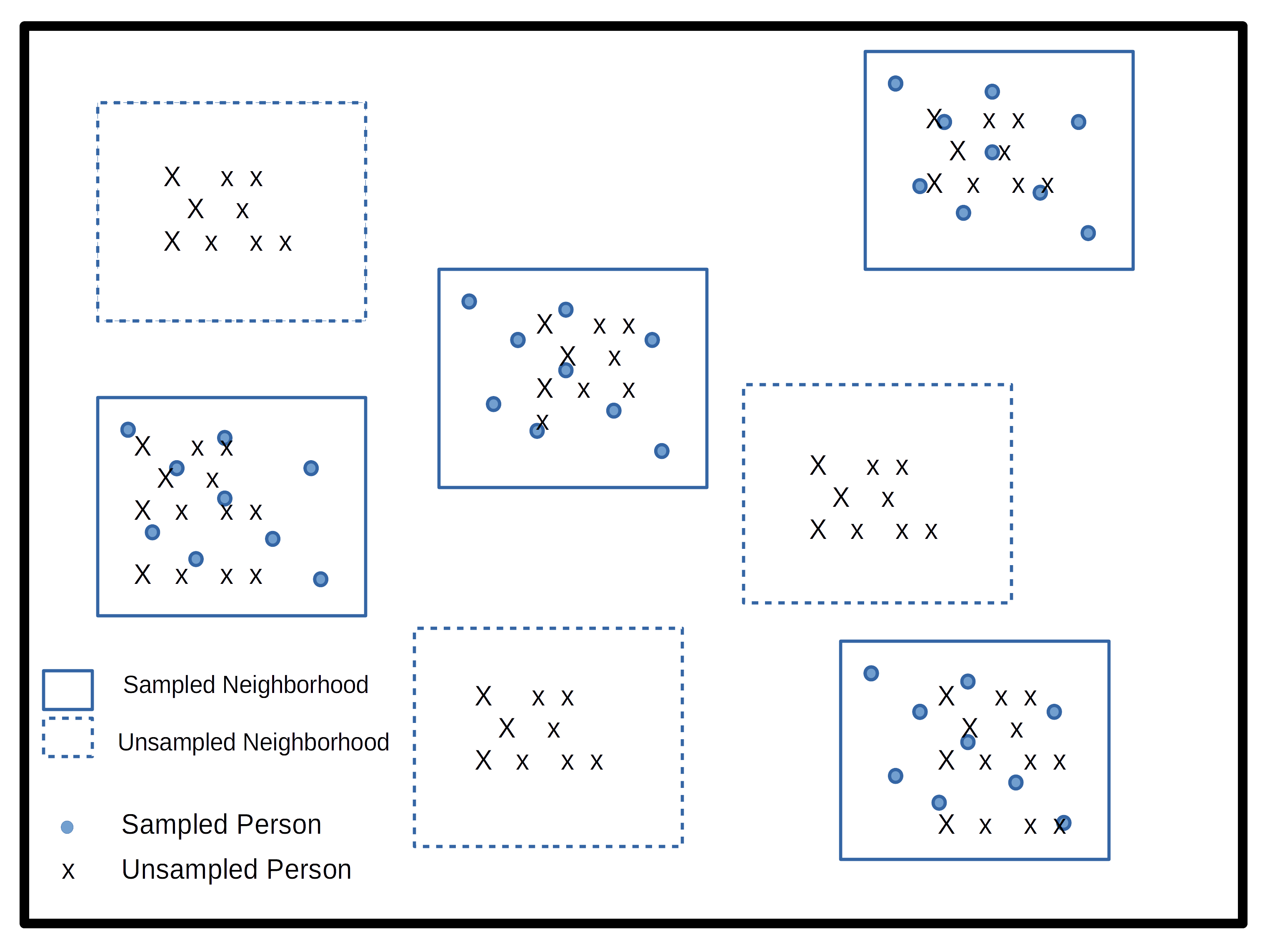
The difference between strata and clusters is easiest to see side by side. In both panels of Figure 2.1 the population is split into the same six groups. A stratified sample takes some people from every group, so every group is guaranteed to be represented. A cluster sample picks a few groups, and then people within only those groups.
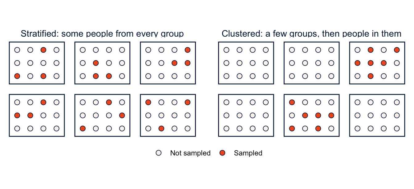
The trouble with clusters is that the people within one are not independent of one another. People in the same village or the same school tend to resemble one another, so 20 people from one village carry less information than 20 people from 20 villages, and clustering usually makes estimates less precise. Nearly every statistical method you learned in the first course assumes independent observations, and a clustered sample violates that assumption by design. Clustering also tends to produce errors that aren’t homoskedastic. So the design has to go into the analysis.
What a weight is
If person \(i\) had a probability \(\pi_i\) of being selected, their base weight is
\[ w_i = \frac{1}{\pi_i} \]
which is the number of people in the population that person stands in for. The \(\pi_i\) is the inclusion probability, and knowing it requires knowing the population. If we stratified the U.S. by rural and urban residence, we’d need to know how many people live in each to know the chance that any one of them is sampled. The more complicated the design, the more complicated the calculation.
Surveys then adjust these base weights for nonresponse and rake or post-stratify them so that weighted totals match known population counts by age, sex, race and ethnicity, and so on. The BRFSS does all of this (Centers for Disease Control and Prevention 2020, 2025). Its design weight combines the stratum weight (which depends on the number of records sampled in a stratum and the density of phone lines there), the number of phones in the household, and the number of adults in the household. That design weight is then raked, adjusted iteratively until the weighted sample matches population margins for age, sex, race and ethnicity, education, marital status, home ownership, phone ownership, and several combinations of these. After all that, a respondent’s weight is interpretable as the number of adults they represent. If your weight is 100, you stand in for 100 people.
He’s not heavy, he’s my brother
The question I get every semester is “Do I really need to weight my analysis?” and of course I say, “Of course!” Weights don’t just inflate your sample up to the size of the population. They correct for the ways the sample differs from the population, and those differences come from three places:
- Unequal probabilities of selection. Some designs give some people a higher chance of selection on purpose. Many surveys oversample small groups so they have enough respondents to say something about them. If recent refugees are 0.1% of a population, a study of refugees might make them 10% of its sample, and the weights then shrink each refugee respondent back down to their share of the population. Add Health, for example, oversampled Black adolescents with college-educated parents, as well as Cuban, Puerto Rican, Chinese and physically disabled adolescents.
- Differences in response rates across groups. Some people are harder to reach or less willing to participate, and nonresponse bias can badly distort population estimates if key groups respond at low rates.
- Differences between the sample and the population that remain after the first two adjustments, which raking and post-stratification fix.
Some surveys are designed to be self-weighting, meaning every unit has the same chance of selection and no weights are needed (or provided). Again, the documentation for your survey tells you which situation you’re in.
With unweighted data, every case counts equally, and the results describe only the people who happened to answer. With weighted data, each case counts in proportion to how many people it represents, and the results describe the target population.
Here is the simplest possible example: five people, with weights.
toy <- tibble(y = c(4, 2, 1, 5, 2),
              weight = c(1, 2, 4, 1, 2))
toy
#> # A tibble: 5 × 2
#> y weight
#> <dbl> <dbl>
#> 1 4 1
#> 2 2 2
#> 3 1 4
#> 4 5 1
#> 5 2 2toy |>
summarise(unweighted_mean = mean(y),
weighted_mean = weighted.mean(y, w = weight))#> # A tibble: 1 × 2
#> unweighted_mean weighted_mean
#> <dbl> <dbl>
#> 1 2.8 2.1The person with y = 1 has a weight of 4, so they count four times as much as the person with y = 4, and the weighted mean is pulled down. That’s all a weight does to a point estimate.
Proportions work the same way, because a proportion is just the mean of a 0/1 variable. Take two respondents. Ana reports fair or poor health (\(y = 1\)) and has a weight of 100. Ben reports good health (\(y = 0\)) and has a weight of 300. The sample proportion is \(1/2 = 0.50\): half of the people who answered are in fair or poor health. The weighted proportion is
\[ \frac{100 \times 1 + 300 \times 0}{100 + 300} = \frac{100}{400} = 0.25 \]
Ana stands in for 100 people and Ben for 300, so of the 400 people they represent, a quarter are in fair or poor health. The 0.50 describes the two respondents. The 0.25 describes the population, as well as two people can.
A weight tells us how much a respondent contributes to the population estimate. A standard error tells us how much that estimate would vary across repeated samples drawn with the same sampling procedure. Correcting the first does not automatically correct the second. That’s the harder part, and the part that takes special software.
The BRFSS SMART MMSA design
Reading the data
get_mmsa() reads the 2024 file and cleans up the names (see the week 1 materials). Keep the calculated variables codebook and the variable layout open while you work.
brfss <- get_mmsa(2024)Finding the design variables
Every survey documents its design variables somewhere, and finding them is always the first job. For the MMSA file there are two: the stratum, _STSTR (ststr after cleaning), and the MMSA final weight, _MMSAWT (mmsawt). The MMSA weight is calibrated to each metro area’s adult population, so it is the right weight for metro-level estimates. Don’t use the state weight from the full BRFSS file with these data.
You might go looking for a cluster variable and not find one. The state BRFSS files include _PSU, but it is just the respondent’s sequence number. The BRFSS samples telephone numbers, not neighborhoods, so each respondent is their own PSU. In survey notation that is ids = ~1.
Writing ids = ~seqno should be equivalent, but it shows a common error.
options(survey.lonely.psu = "adjust")

svydesign(ids = ~seqno, strata = ~ststr, weights = ~mmsawt, data = brfss)
#> Error in `svydesign.default()`:
#> ! Clusters not nested in strata at top level; you may want nest=TRUE.Sequence numbers start over in every state, so the same seqno shows up in more than one stratum. nest = TRUE tells survey that PSU labels are only unique within strata. Many surveys number their PSUs this way, and you will see this error again.
any(duplicated(brfss$seqno))#> [1] TRUEdes_nest <- svydesign(ids = ~seqno, strata = ~ststr, weights = ~mmsawt,
data = brfss, nest = TRUE)
NoteCode explanation:
svydesign() and the ~
svydesign(), from the survey package, builds a design object: the data plus a description of how they were sampled. Every survey function after this takes the design object instead of the data frame.
ids =names the cluster (PSU) variable.~1means “no clusters,” so each respondent is their own PSU.strata =names the stratum variable.weights =names the weight variable.data =is the data frame.nest = TRUEsays that cluster numbers start over in each stratum, so cluster 1 in stratum A and cluster 1 in stratum B are different clusters.
The ~ (tilde) is R’s formula symbol. Here, ~ststr just means “the variable called ststr in the data,” and it lets survey look the variable up inside data without you typing brfss$ststr. You’ll see ~ again in every model this semester, where y ~ x1 + x2 means “model y as a function of x1 and x2.”
any(duplicated(brfss$seqno)) checks the reason for the error: duplicated() marks every value that already appeared earlier in the vector, and any() asks whether at least one is TRUE.
options(survey.lonely.psu = "adjust") changes one of survey’s settings for the rest of the R session, explained next. And #| error: true at the top of the first chunk tells Quarto to show the error and keep rendering, instead of stopping, so you can see what the error looks like.
The survey.lonely.psu option deals with a different problem. A stratum with only one PSU has no within-stratum variance to estimate. The file has 79 strata with a single respondent. Setting the option to "adjust" centers those strata at the overall mean rather than the stratum mean, which is conservative. "average" instead replaces the variance contribution of those strata with the average contribution of all the others. See ?surveyoptions for the rest.
In general, there are three things to find in any survey codebook: the stratum identifier, the PSU (or cluster) identifier, and the respondent weight. Your survey may not have all three, and it may have several weights for different purposes. And be aware that the menu of statistical methods is shorter for complex survey data than for simple random samples. Some analyses you’d like to do may not be available with full design-based inference, and I’ll point out those gaps as we hit them this semester.
Recoding
Now the recodes. Missing value codes (7 for “don’t know”, 9 for “refused”) differ from variable to variable, so check the codebook every time. Here I use the calculated education and age variables, the three-group race and ethnicity measure _RACEGR3, and BMI, which is stored with two implied decimal places.
brfss <- brfss |>
  mutate(
    badhealth = case_when(genhlth %in% 4:5 ~ 1,
                          genhlth %in% 1:3 ~ 0),
    female = if_else(sexvar == 2, 1, 0),
    race_eth = factor(case_when(racegr3 == 1 ~ "NH White",
                                racegr3 == 2 ~ "NH Black",
                                racegr3 == 3 ~ "NH Other",
                                racegr3 == 4 ~ "NH Multiracial",
                                racegr3 == 5 ~ "Hispanic"),
                      levels = c("NH White", "NH Black", "NH Other",
                                 "NH Multiracial", "Hispanic")),
    educ = factor(case_when(educag == 1 ~ "Less than HS",
                            educag == 2 ~ "HS graduate",
                            educag == 3 ~ "Some college",
                            educag == 4 ~ "College graduate"),
                  levels = c("Less than HS", "HS graduate",
                             "Some college", "College graduate")),
    agec = factor(ageg, levels = 1:6,
                  labels = c("18-24", "25-34", "35-44", "45-54", "55-64", "65+")),
    bmi = bmi5 / 100,
    obese = if_else(bmi >= 30, 1, 0),
    texas = str_detect(mmsaname, ", TX"),
    place = str_remove(mmsaname, ", [A-Z]{2}(-[A-Z]{2})*, .*$")
  )
NoteCode explanation:
case_when(), factor() and text patterns
case_when()recodes a variable with a list of rules, each writtencondition ~ value. R checks the rules in order and uses the first one that’s true. Anything that matches no rule becomesNA, which is how the “don’t know” (7) and “refused” (9) codes become missing here without a separate step.genhlth %in% 4:5is true whengenhlthis 4 or 5;%in%asks “is this value one of these?”if_else(condition, yes, no)is the two-outcome version:sexvar == 2gives 1, anything else gives 0.factor(..., levels = ...)turns text into a categorical variable and sets the order of its categories. The first level is the reference category in a regression, so putting “NH White” and “Less than HS” first decides what every coefficient is compared with.factor(ageg, levels = 1:6, labels = ...)does the same for a numeric code, attaching a label to each number.str_detect(mmsaname, ", TX")isTRUEwhen the metro name contains the text “, TX”.str_remove()deletes the part of the text that matches a pattern. The pattern", [A-Z]{2}(-[A-Z]{2})*, .*$"is a regular expression, a small language for describing text. Read it piece by piece: a comma and space, then two capital letters ([A-Z]{2}, a state abbreviation), then optionally more “-XX” state abbreviations ((-[A-Z]{2})*, for metros that cross state lines), then a comma, space, and everything else to the end (.*$). So “San Antonio-New Braunfels, TX, Metropolitan Statistical Area” becomes “San Antonio-New Braunfels”. You won’t need to write patterns like this often; when you do,stringr’s regular expressions vignette is the place to start.
Note
Notice that I recode the whole file and don’t drop anyone yet. Respondents with missing values still carry design information, and when we want estimates for a subgroup, we’ll tell the design about it (more on this below).
Three ways to analyze the same data
I’ll use one question to compare approaches: how does the share of adults reporting fair or poor health differ by education?
Ignoring the design
This is what you get from ordinary tables, which treat the data as a simple random sample.
naive_tab <- table(brfss$badhealth, brfss$educ)
round(100 * prop.table(naive_tab, margin = 2), 1)
#>
#> Less than HS HS graduate Some college College graduate
#> 0 58.0 75.7 79.2 89.0
#> 1 42.0 24.3 20.8 11.0chisq.test(naive_tab)#>
#> Pearson's Chi-squared test
#>
#> data: naive_tab
#> X-squared = 10247, df = 3, p-value < 2.2e-16The gradient is strong: people with less education report worse health. But these are the proportions in the sample, and the test treats every respondent as an independent draw with equal probability of selection. Neither is true.
Weights only
Weighting the table fixes the point estimates.
wt_tab <- xtabs(mmsawt ~ badhealth + educ, data = brfss)
round(100 * prop.table(wt_tab, margin = 2), 1)
#> educ
#> badhealth Less than HS HS graduate Some college College graduate
#> 0 59.8 78.5 81.1 90.1
#> 1 40.2 21.5 18.9 9.9
NoteCode explanation:
table(), prop.table() and xtabs()
table(brfss$badhealth, brfss$educ)counts respondents in each combination of health (rows) and education (columns), as in week 1.prop.table(..., margin = 2)turns counts into proportions within each column (margin = 1would use rows). So each column adds to 1, and we read the share in fair or poor health within each education group.100 *andround(..., 1)make them percentages with one decimal.chisq.test()is the ordinary chi-square test of independence, which assumes a simple random sample.xtabs(mmsawt ~ badhealth + educ)makes the same cross-table with a formula. The variable on the left of the~is added up in each cell, so each cell holds the sum of the weights (the number of adults represented) instead of the number of respondents.
The weighted prevalences are lower than the unweighted ones in every education group. The people who answer the BRFSS are, on average, in worse health than the adult population the weights describe. They’re older, for one thing: 34.1% of respondents are 65 or older, compared with 22.1% of the weighted population. The weights correct for that. This is the “bias” part of the argument for weighting, and it’s why I won’t accept unweighted descriptive statistics from survey data in your papers.
But what about standard errors? For a proportion, the textbook formula is \(s.e.(p) = \sqrt{p(1-p)/n}\), so all we need is \(p\) and \(n\). The trouble is deciding what \(n\) is. In a weighted table, the “count” in each cell is a number of people in the population, not respondents.
wt_se <- as_tibble(wt_tab) |>
  group_by(educ) |>
  mutate(n_weighted = sum(n), p = n / n_weighted) |>
  filter(badhealth == 1) |>
  left_join(count(filter(brfss, !is.na(badhealth)), educ, name = "n_sample"),
            by = "educ") |>
  mutate(se_weighted_n = sqrt(p * (1 - p) / n_weighted),
         se_sample_n = sqrt(p * (1 - p) / n_sample))

wt_se |>
  select(educ, p, n_sample, n_weighted, se_weighted_n, se_sample_n) |>
knitr::kable(digits = c(0, 3, 0, 0, 6, 4), format.args = list(big.mark = ","))| educ | p | n_sample | n_weighted | se_weighted_n | se_sample_n |
|---|---|---|---|---|---|
| Less than HS | 0.402 | 13,303 | 16,334,894 | 0.000121 | 0.0043 |
| HS graduate | 0.215 | 52,247 | 38,917,224 | 0.000066 | 0.0018 |
| Some college | 0.189 | 56,750 | 44,707,055 | 0.000059 | 0.0016 |
| College graduate | 0.099 | 106,381 | 55,939,435 | 0.000040 | 0.0009 |
NoteCode explanation: the standard error table
as_tibble(wt_tab)turns the weighted table into a data frame with one row per cell and the weighted count in a column calledn.group_by(educ)andmutate(n_weighted = sum(n), p = n / n_weighted)add up the weighted counts within each education group and compute the weighted proportion.filter(badhealth == 1)keeps the “fair or poor” rows.left_join(..., by = "educ")adds the number of respondents in each education group, matching rows oneduc. That number comes fromcount(), which counts rows in each group (here, people with non-missing health, by education).- The last
mutate()plugs each version of \(n\) into the textbook formula. knitr::kable()prints a data frame as a formatted table.digitssets the decimals for each column, andformat.args = list(big.mark = ",")adds thousands separators.
If we plug in the weighted \(n\), we’ve basically inflated the sample to the adult population of these metro areas, and the standard errors are absurdly small (the fifth column). Plugging in the number of respondents is better, but that formula still assumes a simple random sample, and as we’re about to see, it is still too small. Getting the right standard error is the other half of what survey software is for.
The full design
Now we declare the design and let survey compute everything.
des <- svydesign(ids = ~1, strata = ~ststr, weights = ~mmsawt, data = brfss)
des
#> Stratified Independent Sampling design (with replacement)
#> svydesign(ids = ~1, strata = ~ststr, weights = ~mmsawt, data = brfss)svyby(~badhealth, ~educ, design = des, FUN = svymean, na.rm = TRUE)#> educ badhealth se
#> Less than HS Less than HS 0.4024662 0.008728778
#> HS graduate HS graduate 0.2147270 0.003619836
#> Some college Some college 0.1886036 0.003383354
#> College graduate College graduate 0.0985978 0.001887432
NoteCode explanation:
svymean(), svyby() and svychisq()
svymean(~badhealth, des) would give the design-based mean of badhealth (the prevalence) for everyone. svyby() repeats a function for each group: the first argument is the variable to summarize, the second the grouping variable, FUN = svymean the function to run in each group, and na.rm = TRUE drops missing values. Printing des shows a short description of the design. svychisq(~badhealth + educ, design = des) is the design-based version of chisq.test(); read its p-value the same way.
The point estimates match the weighted table, and now each one comes with a standard error that reflects the design. The design-based test of independence is the Rao-Scott adjusted chi-square (Rao and Scott 1984), which survey reports as an F statistic.
svychisq(~badhealth + educ, design = des)#>
#> Pearson's X^2: Rao & Scott adjustment
#>
#> data: svychisq(~badhealth + educ, design = des)
#> F = 775.81, ndf = 2.7835e+00, ddf = 6.3863e+05, p-value < 2.2e-16Comparing the standard errors
Standard errors from a survey measure how much an estimate would vary across the many possible samples the design could have drawn. They are what we use to test hypotheses and compare groups, and using inaccurate standard errors can lead us to call results statistically significant when they aren’t, and occasionally the reverse. The usual formulas assume a simple random sample, and software built for simple random samples tends to underestimate the standard errors from complex designs, because it ignores the variation within and between clusters and the effect of unequal weights. There are basically three ways software estimates variances:
- the naive method, which ignores the design;
- Taylor series linearization, which
svydesign()uses by default; and - replication (balanced repeated replication, the jackknife, or the bootstrap), which I come back to at the end of this document.
To see what each piece of the design does, I make two more design objects: one that pretends the data are a simple random sample, and one that uses the weights but ignores the strata.
des_srs <- svydesign(ids = ~1, weights = ~1, data = brfss)
des_wt  <- svydesign(ids = ~1, weights = ~mmsawt, data = brfss)

se_compare <- list("Simple random sample" = des_srs,
                   "Weights only" = des_wt,
                   "Weights and strata" = des) |>
  map(\(d) svyby(~badhealth, ~educ, design = d, FUN = svymean, na.rm = TRUE)) |>
  list_rbind(names_to = "design") |>
  as_tibble() |>
  mutate(design = fct_inorder(design))

se_compare |>
  select(design, educ, badhealth, se) |>
  pivot_wider(names_from = design, values_from = c(badhealth, se)) |>
knitr::kable(digits = 4)| educ | badhealth_Simple random sample | badhealth_Weights only | badhealth_Weights and strata | se_Simple random sample | se_Weights only | se_Weights and strata |
|---|---|---|---|---|---|---|
| Less than HS | 0.4195 | 0.4025 | 0.4025 | 0.0043 | 0.0087 | 0.0087 |
| HS graduate | 0.2430 | 0.2147 | 0.2147 | 0.0019 | 0.0036 | 0.0036 |
| Some college | 0.2082 | 0.1886 | 0.1886 | 0.0017 | 0.0034 | 0.0034 |
| College graduate | 0.1103 | 0.0986 | 0.0986 | 0.0010 | 0.0019 | 0.0019 |
NoteCode explanation:
map() and \(d)
There’s a lot packed into that first pipe, so here it is one step at a time.
list(...)puts the three design objects in a named list. The names are what will label the rows later.map(), frompurrr, runs a function on each element of a list and returns a list of the results. Here it runssvyby()three times, once per design.\(d)is how you write a function on the fly without naming it. It’s shorthand forfunction(d)(added in R 4.1), so it’s the same thing as writingmymean()in week 1, just without saving it. Each time through,map()hands the next design to the function, and inside the function that design is calledd. The name is arbitrary; I useddfor “design.”list_rbind(names_to = "design")stacks the three results into one data frame and adds adesigncolumn with the list names.fct_inorder(design)makesdesigna factor in the order the designs appear, so tables and plots don’t sort them alphabetically.
Without map(), you’d write the svyby() call three times, then label and bind the results yourself:
bind_rows(
  svyby(~badhealth, ~educ, design = des_srs, FUN = svymean, na.rm = TRUE) |> mutate(design = "Simple random sample"),
  svyby(~badhealth, ~educ, design = des_wt,  FUN = svymean, na.rm = TRUE) |> mutate(design = "Weights only"),
  svyby(~badhealth, ~educ, design = des,     FUN = svymean, na.rm = TRUE) |> mutate(design = "Weights and strata")
)
That works, but every copy is a chance for a typo, and adding a fourth design means another copy. You’ll see the same pattern again below, with \(d) { ... } when the function needs more than one line, and \(m) when it loops over models.
se_compare |>
  ggplot(aes(x = educ, y = se, fill = design)) +
  geom_col(position = "dodge") +
  scale_fill_utsa() +
  labs(x = NULL, y = "Standard error", fill = NULL)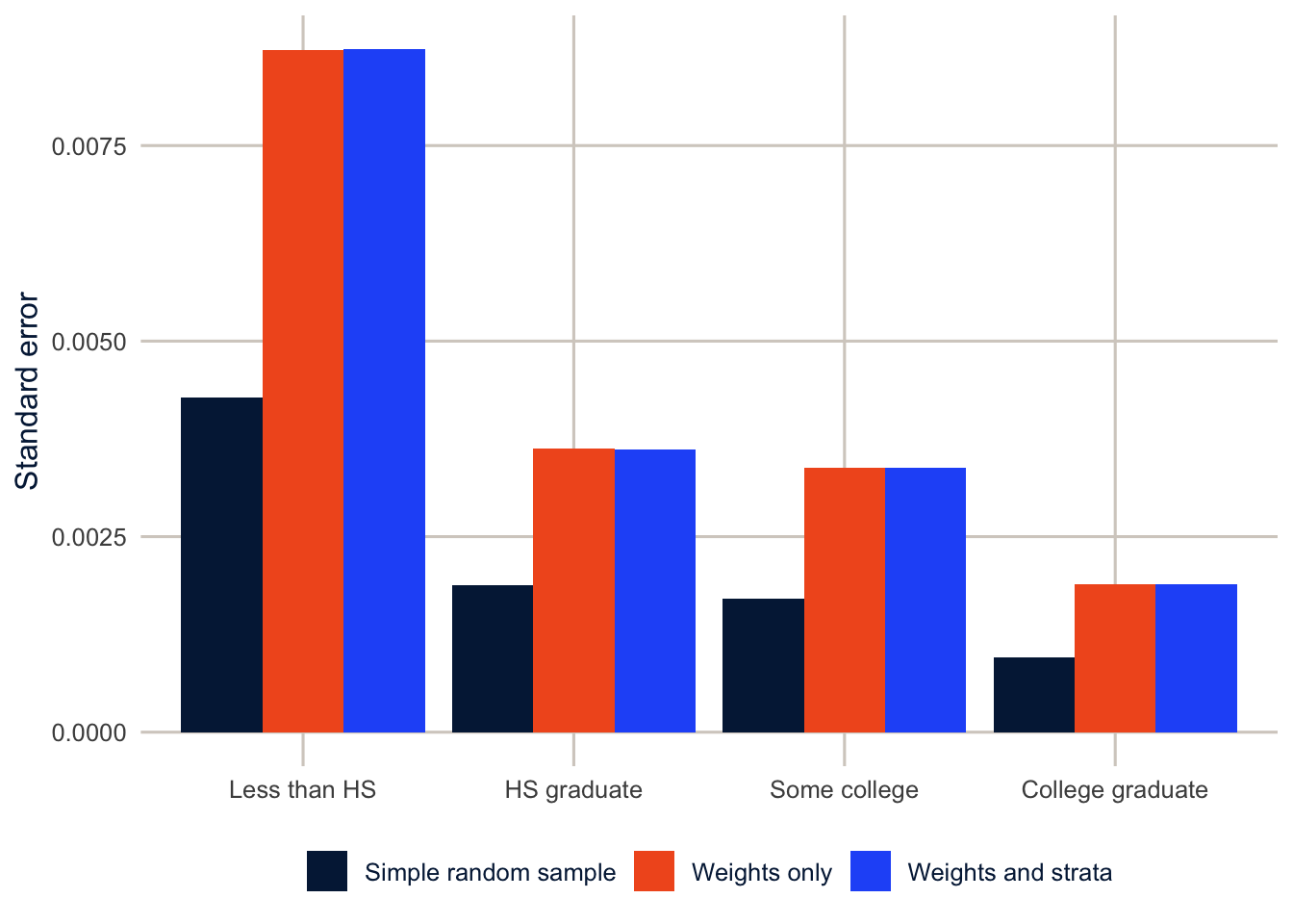
Two things jump out. First, the standard errors from the design are about 1.9 to 2 times larger than the simple random sample ones. Second, almost all of that comes from the weights. Adding the strata barely moves anything (the ratio of the full-design to weights-only standard errors runs from 1 to 1.001).
That is specific to the BRFSS, and I don’t want you to take the wrong lesson from it. In this survey the weights vary a lot, and unequal weights inflate variance. The usual summary of all this is the design effect: the variance of an estimate under the actual design divided by its variance under a simple random sample of the same size. A design effect of 2 means the design doubles the variance (and multiplies the standard error by \(\sqrt{2} \approx 1.41\)). It’s a ratio of variances, and every part of the design feeds into it, so a large design effect doesn’t by itself tell you whether the weights, the strata or the clusters are responsible. Kish (1992) gave a handy approximation for the part due to unequal weights, \(1 + CV^2\) where \(CV\) is the coefficient of variation of the weights, and for the MMSA file it is 4.73. The design effect survey reports for the overall prevalence is 4.86. In other words, our 230,630 respondents carry about as much information as a simple random sample of 47,476. In a clustered survey like the DHS or the ACS, the clusters add their own inflation on top of this.
Don’t take away the idea that a complex design always makes standard errors bigger, though. Stratification usually makes them smaller, because it guarantees the sample covers every stratum, and strata that differ from each other then contribute no sampling variability between them. Clustering and unequal weights usually make them bigger. Which effect wins depends on the survey and on the variable. So the rule doesn’t change: always use the full design, even when it looks like one piece isn’t doing much.
When clusters matter: the DHS
To see what clusters do, I’ll borrow the DHS model dataset, which we’ll use again in weeks 4 and 5. The DHS Program publishes these files so people can learn to use DHS data before applying for access. They describe real households, but no real country. The design variables are the cluster (v021), the stratum (v022) and the women’s weight (v005), which has six implied decimal places. Cluster numbers repeat across strata, so we need nest = TRUE.
dhs <- get_dhs_model() |>
  mutate(wt = v005 / 1e6,
         no_school = as.numeric(v106 == 0),
         rural = as.numeric(v025 == 2),
         modern = as.numeric(v313 == 3))

dhs_designs <- list(
  "Simple random sample" = svydesign(ids = ~1, data = dhs),
  "Weights only" = svydesign(ids = ~1, weights = ~wt, data = dhs),
  "Weights and strata" = svydesign(ids = ~1, strata = ~v022, weights = ~wt, data = dhs),
  "Full design" = svydesign(ids = ~v021, strata = ~v022, weights = ~wt,
                            data = dhs, nest = TRUE)
)

dhs_se <- dhs_designs |>
  map(\(d) {
    est <- svymean(~no_school + modern, d)
    tibble(variable = c("No schooling", "Modern method use"),
           estimate = coef(est), se = SE(est))
  }) |>
  list_rbind(names_to = "design") |>
  mutate(design = fct_inorder(design))

dhs_se |>
  pivot_wider(names_from = variable, values_from = c(estimate, se)) |>
knitr::kable(digits = 4)| design | estimate_No schooling | estimate_Modern method use | se_No schooling | se_Modern method use |
|---|---|---|---|---|
| Simple random sample | 0.5491 | 0.2118 | 0.0054 | 0.0045 |
| Weights only | 0.5267 | 0.2231 | 0.0072 | 0.0063 |
| Weights and strata | 0.5267 | 0.2231 | 0.0066 | 0.0062 |
| Full design | 0.5267 | 0.2231 | 0.0169 | 0.0142 |
Here the story is different. The 8,348 women in the file live in 217 clusters, and adding the clusters to the design multiplies the standard error of the share with no schooling by 2.5. The design effect is 9.5, so this sample carries about as much information about schooling as a simple random sample of 875 women. The design effect for modern contraceptive use is about as large, 9.7. The design effects alone don’t say why the variance is larger, but the table does: the standard errors jump when the clusters are added, not when the weights or strata are. So here the clustering is what’s doing it, and both variables are strongly clustered. Whether a woman went to school depends a great deal on where she grew up, and whether she uses a modern method depends on what services are nearby and what her neighbors do, so women in the same cluster tend to look alike on both. Compare that with the BRFSS, where every respondent is their own PSU and the design effect came almost entirely from the weights.
The same thing happens in regression. Here is a linear model for the number of children ever born, fit as if the data were a simple random sample and then with the full design.
f_ceb <- v201 ~ v012 + I(v012^2) + no_school + rural

fit_dhs_lm <- lm(f_ceb, data = dhs)
fit_dhs_svy <- svyglm(f_ceb, design = dhs_designs[["Full design"]])

tibble(term = names(coef(fit_dhs_lm)),
       estimate_ols = coef(fit_dhs_lm),
       estimate_svy = coef(fit_dhs_svy),
       se_ols = sqrt(diag(vcov(fit_dhs_lm))),
       se_svy = SE(fit_dhs_svy)) |>
  mutate(ratio = se_svy / se_ols) |>
knitr::kable(digits = 3)| term | estimate_ols | estimate_svy | se_ols | se_svy | ratio |
|---|---|---|---|---|---|
| (Intercept) | -4.933 | -4.865 | 0.183 | 0.264 | 1.442 |
| v012 | 0.313 | 0.304 | 0.013 | 0.023 | 1.759 |
| I(v012^2) | -0.002 | -0.002 | 0.000 | 0.000 | 1.669 |
| no_school | 0.618 | 0.747 | 0.044 | 0.098 | 2.245 |
| rural | 0.497 | 0.625 | 0.039 | 0.094 | 2.408 |
NoteCode explanation: formulas,
svyglm() and pulling results out of a model
f_ceb <- v201 ~ v012 + I(v012^2) + no_school + ruralsaves a model formula in an object so both models use exactly the same one.v201(children ever born) is the outcome;v012is age.I(v012^2)adds age squared. Inside a formula,^has a special meaning, soI()(“as is”) tells R to do ordinary arithmetic: square age, and use that as a predictor. Age plus age squared lets the line curve.lm()fits the model by ordinary least squares, ignoring the design.svyglm(formula, design = ...)fits a regression with the survey design: weighted estimates and design-based standard errors. It works likeglm(), so you’ll use it for logit and count models in later weeks too.coef()extracts the coefficients from a model.vcov()extracts their variance-covariance matrix; the variances are on its diagonal, sosqrt(diag(vcov(...)))gives the standard errors.SE()does the same in one step forsurveyobjects.
The coefficients differ a little because of the weights, and the standard errors from the design are larger, most of all for the two variables that are measured at, or strongly patterned by, the cluster. Rural residence is the extreme case: every woman in a cluster has the same value, so the effective sample size for that coefficient is closer to the number of clusters than to the number of women. This is the same logic as clustered standard errors in econometrics (Cameron and Miller 2015), and it’s why it is commonplace for a survey model to give larger p-values than a naive one.
Subpopulations: subset the design, don’t filter the data
Start with the question. Suppose we want to know what share of Hispanic adults in San Antonio are obese. The population is now a subgroup, but the sample wasn’t drawn from Hispanic San Antonians. It was drawn from everyone, and the number of Hispanic San Antonians who ended up in it is itself random: a different sample would have had a different number. A correct standard error has to reflect that randomness, so the design needs to know about the whole sample, not just the people in the subgroup.
So the tempting move, filtering the data and building a design from what’s left, is wrong. The right move is to build the design on the full data and then subset() it. The design-based variance depends on how many respondents fall in each stratum, and a subset keeps track of that while a filtered data frame forgets it.
sa_hisp <- brfss$race_eth %in% "Hispanic" & str_detect(brfss$place, "^San Antonio")

# the right way
svymean(~obese, subset(des, sa_hisp), na.rm = TRUE)
#> mean SE
#> obese 0.39143 0.0291# the tempting way
svydesign(ids = ~1, strata = ~ststr, weights = ~mmsawt,
data = filter(brfss, sa_hisp)) |>
svymean(~obese, design = _, na.rm = TRUE)#> mean SE
#> obese 0.39143 0.029
NoteCode explanation:
subset() and the _ placeholder
sa_hisp is a vector of TRUE and FALSE, one per respondent. & means “and,” so it’s TRUE only for people who are Hispanic and live in San Antonio. subset(des, sa_hisp) keeps the full design but marks only those people as the subpopulation.
In the second version, the pipe |> normally passes the result on as the first argument of the next function. svymean()’s first argument is the formula, not the design, so design = _ says “put the result here instead.” The _ placeholder only works with a named argument.
In fairness, the two answers here are nearly identical. Because every BRFSS respondent is their own PSU, filtering loses very little. In a clustered design the filtered version can be badly wrong, and filtering can also leave strata with a single PSU, which breaks the variance calculation. So subset() is the habit to build. srvyr does the same thing when you call filter() on a survey object (not on the data frame), which is one reason I like it.
Descriptive tables
srvyr puts the design inside a dplyr pipeline. Grouping and summarizing work the way you’d expect, and survey_mean() returns the standard error (or a confidence interval) along with the estimate.
brfss_svy <- brfss |>
  as_survey_design(ids = 1, strata = ststr, weights = mmsawt)

brfss_svy |>
  filter(!is.na(educ)) |>
  group_by(educ, female) |>
  summarise(badhealth = survey_mean(badhealth, na.rm = TRUE, vartype = "ci"))
#> # A tibble: 8 × 5
#> # Groups: educ [4]
#> educ female badhealth badhealth_low badhealth_upp
#> <fct> <dbl> <dbl> <dbl> <dbl>
#> 1 Less than HS 0 0.384 0.360 0.407
#> 2 Less than HS 1 0.422 0.397 0.447
#> 3 HS graduate 0 0.201 0.192 0.211
#> 4 HS graduate 1 0.229 0.219 0.239
#> 5 Some college 0 0.178 0.169 0.187
#> 6 Some college 1 0.198 0.188 0.207
#> 7 College graduate 0 0.0954 0.0904 0.100
#> 8 College graduate 1 0.101 0.0961 0.107
NoteCode explanation:
as_survey_design() and survey_mean()
as_survey_design() is srvyr’s version of svydesign(). The arguments are the same, but you write variable names without the ~, and ids = 1 means no clusters. After that you use the ordinary dplyr verbs on the design. survey_mean() works like mean() inside summarise(), but it uses the weights and adds a design-based standard error, or a confidence interval with vartype = "ci" (the _low and _upp columns).
For a paper, gtsummary builds the familiar “Table 1” from a survey design, with weighted percentages and design-based tests.
brfss_svy |>
  filter(!is.na(educ)) |>
  select(educ, badhealth, obese, race_eth, agec) |>
  tbl_svysummary(by = educ,
                 label = list(badhealth ~ "Fair or poor health",
                              obese ~ "Obese (BMI 30 or more)",
                              race_eth ~ "Race and ethnicity",
                              agec ~ "Age group"),
                 statistic = list(all_categorical() ~ "{p}%"),
                 missing = "no") |>
  add_p() |>
  modify_spanning_header(all_stat_cols() ~ "**Educational attainment**") |>
bold_labels()| Characteristic |
Educational attainment
|
p-value2 | |||
|---|---|---|---|---|---|
| Less than HS N = 16,422,9161 |
HS graduate N = 39,046,0311 |
Some college N = 44,796,8161 |
College graduate N = 56,030,5441 |
||
| Fair or poor health | 40% | 21% | 19% | 9.9% | <0.001 |
| Obese (BMI 30 or more) | 37% | 33% | 34% | 26% | <0.001 |
| Race and ethnicity | <0.001 | ||||
| NH White | 23% | 50% | 55% | 60% | |
| NH Black | 10% | 16% | 16% | 11% | |
| NH Other | 4.3% | 7.2% | 7.7% | 15% | |
| NH Multiracial | 1.7% | 2.3% | 3.2% | 2.3% | |
| Hispanic | 61% | 24% | 18% | 12% | |
| Age group | <0.001 | ||||
| 18-24 | 12% | 21% | 13% | 4.8% | |
| 25-34 | 15% | 16% | 16% | 19% | |
| 35-44 | 18% | 14% | 15% | 21% | |
| 45-54 | 16% | 13% | 15% | 18% | |
| 55-64 | 17% | 14% | 16% | 16% | |
| 65+ | 21% | 22% | 24% | 21% | |
| 1 | |||||
| 2 Pearson’s X^2: Rao & Scott adjustment | |||||
NoteCode explanation:
tbl_svysummary()
tbl_svysummary() builds a descriptive table from a survey design. by = educ makes one column per education group. label gives each variable a readable name, using the variable ~ "label" formula style. statistic = list(all_categorical() ~ "{p}%") shows weighted percentages for every categorical variable. missing = "no" leaves out the count of missing values. Then add_p() adds a design-based test for each row, modify_spanning_header() puts a heading over the group columns, and bold_labels() bolds the variable names.
The percentages are weighted, and the p-values come from Rao-Scott tests. This is the kind of descriptive table you should report. gtsummary is built on the gt package (Iannone et al., n.d.), which builds tables in much the same layered way ggplot2 builds plots, so anything you can do to a gt table (footnotes, column formats, colors) you can do to these. Because a srvyr pipeline always ends in a data frame, gt() or knitr::kable() will also print any of the summaries above as a table, and that keeps every number in your paper tied to the code that made it, with no copying from the console into Word.
Regression with survey data
The same logic carries over to regression. I’ll fit a linear model for BMI three ways: ordinary least squares, least squares with the weights, and svyglm() with the full design.
f_bmi <- bmi ~ educ + agec + female + race_eth

fit_ols <- lm(f_bmi, data = brfss)
fit_wls <- lm(f_bmi, data = brfss, weights = mmsawt)
fit_svy <- svyglm(f_bmi, design = des, family = gaussian())

modelsummary(list("OLS" = fit_ols,
                  "Weighted OLS" = fit_wls,
                  "Survey design" = fit_svy),
             gof_map = "nobs",
             fmt = 3,
             coef_rename = \(x) str_remove_all(x, "educ|agec|race_eth"),
title = "Linear models for BMI, 2024 BRFSS SMART MMSA")| OLS | Weighted OLS | Survey design | |
|---|---|---|---|
| (Intercept) | 26.007 | 26.074 | 26.074 |
| (0.086) | (0.070) | (0.262) | |
| HS graduate | -0.083 | -0.356 | -0.356 |
| (0.070) | (0.057) | (0.214) | |
| Some college | -0.122 | -0.393 | -0.393 |
| (0.070) | (0.057) | (0.208) | |
| College graduate | -1.344 | -1.625 | -1.625 |
| (0.068) | (0.056) | (0.201) | |
| 25-34 | 2.698 | 2.780 | 2.780 |
| (0.068) | (0.056) | (0.147) | |
| 35-44 | 3.642 | 3.569 | 3.569 |
| (0.066) | (0.056) | (0.149) | |
| 45-54 | 4.175 | 3.979 | 3.979 |
| (0.066) | (0.057) | (0.161) | |
| 55-64 | 3.763 | 3.657 | 3.657 |
| (0.064) | (0.057) | (0.151) | |
| 65+ | 2.436 | 2.422 | 2.422 |
| (0.060) | (0.053) | (0.136) | |
| female | -0.077 | -0.058 | -0.058 |
| (0.028) | (0.029) | (0.068) | |
| NH Black | 1.474 | 1.371 | 1.371 |
| (0.048) | (0.044) | (0.102) | |
| NH Other | -1.301 | -1.705 | -1.705 |
| (0.066) | (0.052) | (0.115) | |
| NH Multiracial | 0.395 | 0.165 | 0.165 |
| (0.100) | (0.093) | (0.195) | |
| Hispanic | 0.489 | 0.613 | 0.613 |
| (0.046) | (0.040) | (0.107) | |
| Num.Obs. | 203383 | 203383 | 203383 |
NoteCode explanation: weighted
lm(), svyglm() and modelsummary()
lm(f_bmi, data = brfss, weights = mmsawt)passes the survey weights tolm(). As explained below,lm()treats them as a different kind of weight, which is the point of the comparison.svyglm(f_bmi, design = des, family = gaussian())fits the same linear model with the design.family = gaussian()makes it an ordinary linear regression (it’s the default, and later weeks change it tobinomial()for logits andpoisson()for counts).modelsummary()puts several models side by side. Give it a namedlist(), and the names become the column headings.gof_map = "nobs"shows only the number of observations at the bottom,fmt = 3rounds to three decimals, andcoef_renamecleans up the coefficient names with a small function:str_remove_all(x, "educ|agec|race_eth")deletes the variable-name prefixes R adds to each category (|means “or” in a pattern), soeducHS graduateis shown asHS graduate.
The weighted model and the survey model have identical coefficients, and they differ from OLS because the weights change whose BMI we’re describing. The standard errors are the interesting part. lm() with weights treats the weights as precision weights, which is a different statistical idea altogether, and its standard errors are not right for survey data. svyglm() uses a sandwich (robust) variance estimator that accounts for the weights and the design, the same family of estimators economists use for clustered data (Cameron and Miller 2015).
coefs <- list("OLS" = fit_ols,
              "Weighted OLS" = fit_wls,
              "Survey design" = fit_svy) |>
  map(\(m) broom::tidy(m, conf.int = TRUE)) |>
  list_rbind(names_to = "model") |>
  filter(term != "(Intercept)") |>
  mutate(model = fct_inorder(model),
         term = str_remove_all(term, "educ|agec|race_eth"),
         term = fct_inorder(term))

coefs |>
  ggplot(aes(x = estimate, y = fct_rev(term), colour = model, shape = model)) +
  geom_vline(xintercept = 0, colour = utsa_cols("smoke")) +
  geom_pointrange(aes(xmin = conf.low, xmax = conf.high),
                  position = position_dodge(width = 0.6)) +
  scale_colour_utsa() +
  labs(x = "Difference in BMI", y = NULL, colour = NULL, shape = NULL)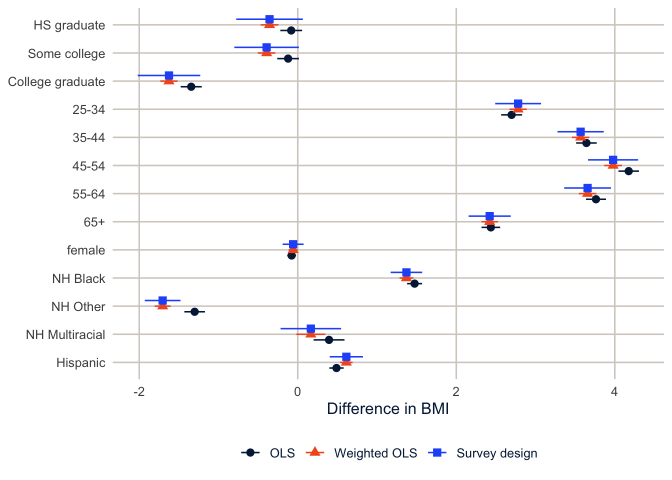
NoteCode explanation: a coefficient plot
broom::tidy(m, conf.int = TRUE) turns a fitted model into a data frame with one row per coefficient: term, estimate, std.error, p.value, and the confidence limits conf.low and conf.high. The rest of the pipe stacks the three models, as in the map() example earlier. In the plot, geom_pointrange() draws each estimate as a point with a line for its interval, position_dodge() sets the three models side by side instead of on top of each other, and fct_rev(term) reverses the order of the terms so the first coefficient is at the top. geom_vline(xintercept = 0) draws the line for “no difference.”
The survey standard errors are 1.7 to 3.1 times the OLS ones. With 203,383 respondents most of these effects stay clearly different from zero either way, and the big picture (BMI is lower among college graduates and peaks in middle age) doesn’t change. But look at the coefficient for women. OLS says women’s BMI is 0.08 points lower, with p = 0.0068. The survey model puts the difference at 0.06 points with p = 0.39. Same data, same model, and the “finding” goes away once the standard error reflects the design. With a smaller sample or a smaller effect this happens often, so fit the right model from the start.
Estimates for places
The point of the SMART file is estimates for metro areas. svyby() with svyciprop() gives prevalences with confidence intervals computed on the logit scale, which stay inside 0 and 1 for small groups.
tx_fit <- svyby(~obese, ~place, design = subset(des, texas),
                FUN = svyciprop, vartype = c("se", "ci"), na.rm = TRUE)

tx_obesity <- tibble(place = tx_fit$place,
                     obese = coef(tx_fit),
                     se = SE(tx_fit),
                     ci_l = tx_fit$ci_l,
                     ci_u = tx_fit$ci_u) |>
  left_join(brfss |>
              filter(texas, !is.na(obese)) |>
              count(place, name = "n"),
            by = "place") |>
  mutate(rse = se / obese) |>
  relocate(n, .after = place) |>
  arrange(desc(obese))

knitr::kable(tx_obesity, digits = 3, format.args = list(big.mark = ","))| place | n | obese | se | ci_l | ci_u | rse |
|---|---|---|---|---|---|---|
| Beaumont-Port Arthur | 454 | 0.425 | 0.039 | 0.351 | 0.503 | 0.091 |
| San Antonio-New Braunfels | 1,287 | 0.362 | 0.018 | 0.327 | 0.399 | 0.050 |
| Houston-Pasadena-The Woodlands | 1,531 | 0.360 | 0.024 | 0.314 | 0.408 | 0.066 |
| Fort Worth-Arlington-Grapevine | 986 | 0.360 | 0.023 | 0.316 | 0.405 | 0.063 |
| Dallas-Plano-Irving | 1,420 | 0.324 | 0.017 | 0.292 | 0.359 | 0.053 |
| Austin-Round Rock-San Marcos | 941 | 0.287 | 0.020 | 0.249 | 0.327 | 0.069 |
NoteCode explanation:
svyciprop()
svyciprop() estimates a proportion with a confidence interval designed for proportions, which stays between 0 and 1 even for small groups. Inside svyby(), vartype = c("se", "ci") asks for both the standard error and the interval. The tibble() call then pulls the pieces out of the result: coef() the estimates, SE() the standard errors, and ci_l and ci_u the interval limits. relocate(n, .after = place) moves the respondent count next to the place name, and arrange(desc(obese)) sorts from highest to lowest.
tx_obesity |>
  mutate(place = fct_reorder(place, obese),
         highlight = str_detect(place, "^San Antonio")) |>
  ggplot(aes(x = obese, y = place, colour = highlight)) +
  geom_pointrange(aes(xmin = ci_l, xmax = ci_u), linewidth = 1, size = 0.6) +
  scale_colour_manual(values = c(`FALSE` = utsa_cols("midnight")[[1]],
                                 `TRUE` = utsa_cols("orange")[[1]]),
                      guide = "none") +
  scale_x_continuous(labels = scales::label_percent()) +
  labs(x = "Obesity prevalence (BMI 30 or more)", y = NULL)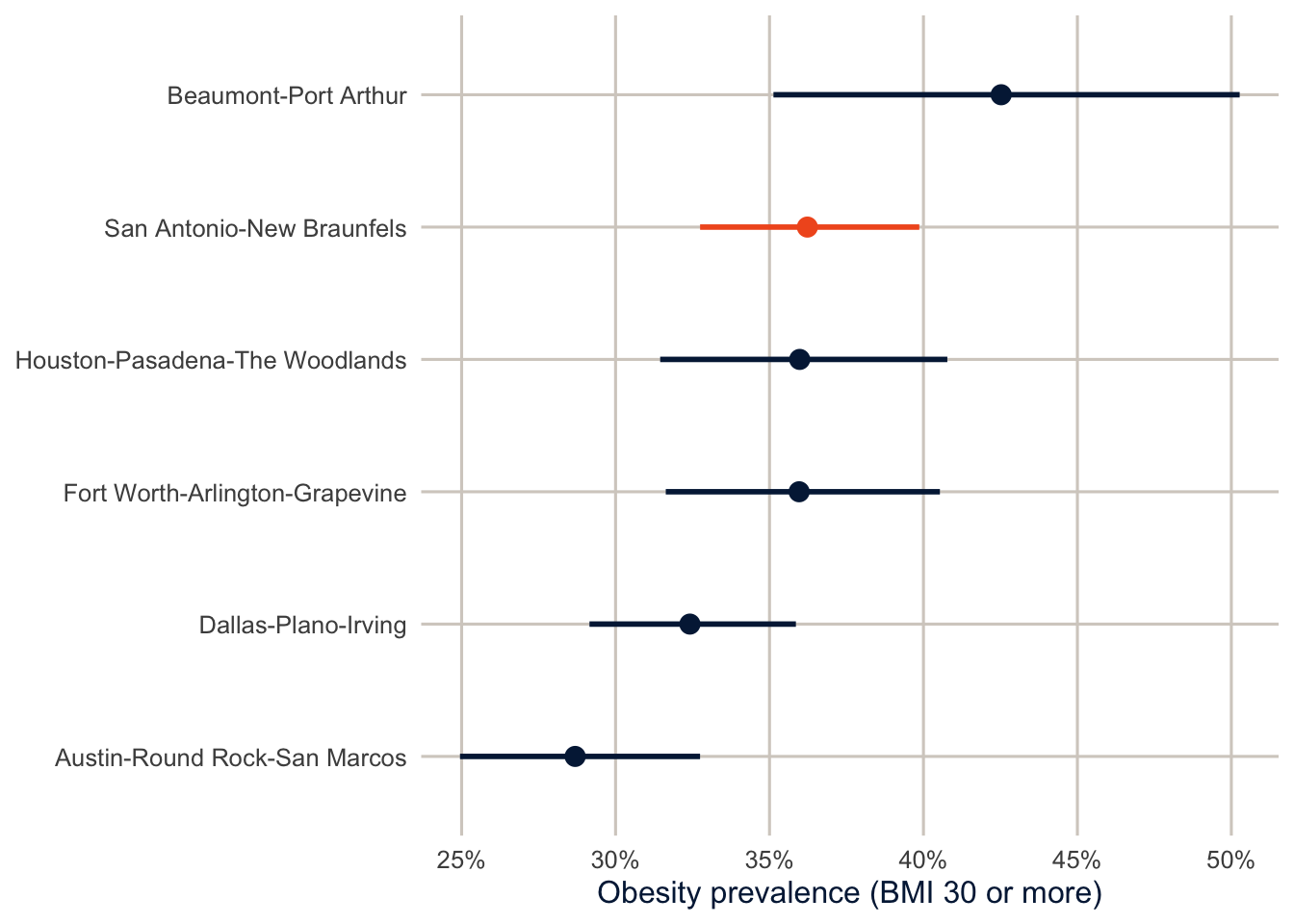
Look at Beaumont-Port Arthur. It has the highest estimate, 42.5%, but it also has the fewest respondents (454) and by far the widest interval, from 35.1% to 50.3%. That interval overlaps every other Texas metro except Austin, so “Beaumont has the highest obesity rate in Texas” is a claim these data can’t support. (Overlapping intervals are a rough screen, not a test. Two intervals can overlap a little even when the difference between the groups is statistically significant. To compare two places properly, estimate the difference and its confidence interval, which svycontrast() does.) CDC suppresses MMSA estimates that rest on too few respondents or have intervals that are too wide, and you should check the methodology document for the current rule before you publish a metro-level number (Centers for Disease Control and Prevention 2025). The relative standard error (the rse column, the standard error divided by the estimate) is a quick screen. Many agencies flag estimates with an RSE above 0.30.
TipReading the result: a right and a wrong interpretation
Right: “An estimated 42.5% of adults in the Beaumont-Port Arthur metro area are obese (95% confidence interval 35.1% to 50.3%), based on 454 respondents to the 2024 BRFSS.”
Wrong: “42.5% of the Beaumont-Port Arthur respondents are obese.” The weighted estimate isn’t the share of the respondents; it’s an estimate for the adult population they represent, and the share among the respondents themselves could be quite different. The right version also gives the interval and the number of respondents, so a reader can see how much to trust it.
One of the most useful things about the SMART file is that we can go a step further and estimate prevalences for demographic groups within places. svyby() takes more than one grouping variable, so here is obesity by sex in each Texas metro.
tx_sex <- svyby(~obese, ~place + female, design = subset(des, texas),
                FUN = svymean, na.rm = TRUE)

as_tibble(tx_sex) |>
  mutate(sex = if_else(female == 1, "Women", "Men"),
         rse = se / obese) |>
  select(place, sex, obese, se, rse) |>
  pivot_wider(names_from = sex, values_from = c(obese, se, rse)) |>
knitr::kable(digits = 3)| place | obese_Men | obese_Women | se_Men | se_Women | rse_Men | rse_Women |
|---|---|---|---|---|---|---|
| Austin-Round Rock-San Marcos | 0.276 | 0.298 | 0.025 | 0.031 | 0.089 | 0.105 |
| Beaumont-Port Arthur | 0.461 | 0.389 | 0.063 | 0.043 | 0.137 | 0.111 |
| Dallas-Plano-Irving | 0.301 | 0.348 | 0.023 | 0.025 | 0.076 | 0.073 |
| Fort Worth-Arlington-Grapevine | 0.342 | 0.378 | 0.030 | 0.035 | 0.087 | 0.092 |
| Houston-Pasadena-The Woodlands | 0.354 | 0.366 | 0.031 | 0.036 | 0.088 | 0.100 |
| San Antonio-New Braunfels | 0.335 | 0.391 | 0.025 | 0.027 | 0.074 | 0.068 |
Each cell has fewer respondents than the place as a whole, so the standard errors grow, and the RSE screen matters more the finer you slice the data. The Texas metros are large enough that every sex-specific estimate here stays well under an RSE of 0.30, though Beaumont-Port Arthur’s are noticeably less precise than the rest. Split these cells again by race and ethnicity or by age, and many of them won’t pass.
Replicate weights
So far survey has used Taylor series linearization to get standard errors. It approximates the variance of whatever we’re estimating (a ratio, a regression coefficient) with a linear function whose variance we know how to compute from the strata and PSUs. It works well and it’s the default for most software.
The other approach is replication. Replicate weights are repeated, carefully constructed versions of the analysis weight, each one a little different. You compute your estimate once with the main weight, then again with each replicate weight, and use the spread of those estimates as the standard error. You don’t need to know how the agency built them to use them, only which formula the documentation says to use. The perturbations take a few common forms:
- Balanced repeated replication (BRR), for designs with two PSUs per stratum, which keeps one PSU from each stratum in each replicate.
- The jackknife, which drops one PSU (or a group of them) at a time and reweights the rest.
- The bootstrap, which resamples PSUs with replacement within strata.
- Successive difference replication (SDR), which the Census Bureau uses for the ACS and the CPS.
Replication has two big advantages. The weights can carry things a strata-and-PSU description can’t, like the adjustments that line the sample up with census totals, and they let agencies publish design information without publishing strata and PSU codes that could help identify respondents. That second reason is why so many public-use files come with replicate weights and nothing else. You’ll sometimes read that replication also takes care of statistics that are hard to linearize, like medians. That’s true for the bootstrap and BRR, but the jackknife needs more care, and so do the ACS replicates, as we’ll see below.
Data that come with replicate weights: the ACS
The ACS public use microdata sample (PUMS) has no strata or PSU variables. It has a person weight, PWGTP, and 80 replicate weights, PWGTP1 through PWGTP80, built with successive difference replication. tidycensus downloads them (you’ll need a free Census API key, set with census_api_key()), and to_survey() builds the replicate design with the scale factor the Census Bureau documents for these weights. The download is large, so I save a copy the first time.
acs_file <- here("data", "acs_pums_tx2024.rds")

if (!file.exists(acs_file)) {
  tx_pums <- get_pums(variables = c("AGEP", "SEX", "POVPIP"),
                      state = "TX",
                      survey = "acs1",
                      year = 2024,
                      rep_weights = "person")
  saveRDS(tx_pums, acs_file)
}
tx_pums <- readRDS(acs_file)
acs_svy <- tx_pums |>
mutate(age = as.numeric(AGEP),
povpip = as.numeric(POVPIP),
# POVPIP is income as a percent of the poverty line; -1 means not determined
poverty = case_when(povpip < 0 ~ NA_real_,
povpip < 100 ~ 1,
.default = 0),
age65 = as.numeric(age >= 65)) |>
to_survey(type = "person", design = "rep_weights")
acs_svy#> Call: Called via srvyr
#> Unstratified cluster jacknife (JK1) with 80 replicates and MSE variances.
#> Data variables:
#> - SERIALNO (chr), SPORDER (dbl), AGEP (dbl), POVPIP (dbl), STATE (chr), SEX
#> (chr), WGTP (dbl), age (dbl), povpip (dbl), poverty (dbl), age65 (dbl)
NoteCode explanation:
get_pums() and to_survey()
get_pums(), from tidycensus, downloads ACS microdata: the variables you name, for one state, survey ("acs1" is the one-year file), and year. rep_weights = "person" includes the 80 person replicate weights. if (!file.exists(acs_file)) { ... } only runs the download when there’s no saved copy yet (! means “not”), and saveRDS() and readRDS() save and read that copy.
In the next chunk, case_when() codes poverty, with .default = 0 for everyone not matched by an earlier rule, and to_survey() builds a srvyr replicate design using the formula the Census Bureau documents. survey_total() (below) estimates a population total, the way survey_mean() estimates a mean.
acs_est <- acs_svy |>
  summarise(population = survey_total(),
            poverty_rate = survey_mean(poverty, na.rm = TRUE),
            share_65plus = survey_mean(age65))
acs_est
#> # A tibble: 1 × 6
#> population population_se poverty_rate poverty_rate_se share_65plus
#> <dbl> <dbl> <dbl> <dbl> <dbl>
#> 1 31290831 0 0.134 0.00162 0.140
#> # ℹ 1 more variable: share_65plus_se <dbl>The printout calls this a JK1 design with 80 replicates. That is just how survey labels the variance formula: the Census Bureau’s formula for these weights is \(\frac{4}{80}\sum_{r=1}^{80}(\hat\theta_r - \hat\theta)^2\), and to_survey() sets the JK1 scale to \(4/80\) so the two are the same.
The weighted total puts the Texas population at 31.3 million, with a standard error of 0. That isn’t a bug. The ACS weights, including every replicate weight, are controlled to the Census Bureau’s official population estimates, so they all add up to the same total and the total has no sampling variance. Totals for subgroups that aren’t part of the controls (people in poverty, for example) do have sampling error. The poverty rate is 13.4% with a standard error of 0.16 percentage points. If we ignored the design entirely, the unweighted rate in the sample would be 12.0% and the textbook standard error, \(\sqrt{p(1-p)/n}\), would be 0.06 points. The replicate standard error is the one to report, and it is what the Census Bureau’s own published margins of error are built from (a 90% MOE is 1.645 times the standard error).
Tip
Every survey documents its replicate method, the number of replicates, and the scale factor. tidycensus knows these for the ACS. For other surveys you’ll set them yourself with svrepdesign() or as_survey_rep(), using the type, scale, rscales and mse arguments, and you should copy them from the codebook, not from someone else’s code (including mine).
The same data from IPUMS
The ACS microdata are also available from the Integrated Public Use Microdata Series (IPUMS) at the University of Minnesota (Ruggles et al. 2025), which adds harmonized variables and makes it much easier to work across years. The IPUMS version adds two design variables of its own, STRATA and CLUSTER, built from the ACS sampling strata and the households within them, so you can use either a linearization design or the replicate weights (REPWTP1 to REPWTP80 for people, REPWT1 to REPWT80 for households).
For this example I made an IPUMS USA extract of the 2024 one-year ACS with the design variables, the person and household weights, all 80 person replicate weights, and some demographic, education, work and income variables. The extract covers the whole country, and the compressed data file is over half a gigabyte, so I kept only the Texas records, and that’s the file in the data folder. When you make your own extract, the “Select cases” option on the IPUMS site does the same thing before you download, and it’s where you decide whether to include people living in group quarters (dorms, prisons, nursing homes). Mine has people in households only.
An IPUMS download comes in two pieces: the data file (.dat.gz) and a codebook in a format called DDI (.xml). ipumsr reads them together.
ddi <- read_ipums_ddi(here("data", "usa_00014.xml"))
ipums <- read_ipums_micro(ddi, data_file = here("data", "usa_00014_tx.dat.gz"),
                          verbose = FALSE)
dim(ipums)
#> [1] 278666 120
NoteCode explanation: reading IPUMS data with
ipumsr
The .dat.gz file is a compressed fixed-width text file. There are no commas or tabs between values. Each variable sits in the same columns on every line (STATEFIP is always characters 55 and 56, for example), so the data file is just a wall of digits until something tells R where each variable starts and stops. That’s the DDI’s job.
read_ipums_ddi()reads the codebook: the variable names, their column positions, their labels and the labels for every code.read_ipums_micro(ddi)uses the codebook to read the data. Normally it looks for a data file with the same name as the DDI in the same folder. My Texas file has a different name, so I point to it withdata_file. With your own extract, keep the two files together and you can leavedata_fileout.verbose = FALSEturns off the message asking you to cite IPUMS. Cite it anyway; they ask you to, and it’s how they keep their funding.
The result is a data frame with one row per person and variable names in capitals, the way IPUMS writes them. Many columns are labelled: they store the numeric code, with the label attached. as_factor() turns the codes into their labels, and ipums_val_labels() prints the whole code list for a variable. The R script IPUMS gives you with each extract (see R/usa_00014.R) does the same two steps, without the data_file argument.
As always, check the codebook before using a variable. In IPUMS, INCWAGE stores “N/A” (people too young to be asked, or without wages) as 999999, and missing as 999998. Take the mean of INCWAGE without recoding those, and the average wage in Texas comes out to $217,849.
ipums_val_labels(ipums$INCWAGE)#> # A tibble: 9 × 2
#> val lbl
#> <dbl> <chr>
#> 1 1940 top code: $5,001
#> 2 1950 top code: $10,000
#> 3 1960 top code: $25,000
#> 4 1970 top code: $50,000
#> 5 1980 top code: $75,000
#> 6 1990 top code: $140,000*
#> 7 2000 top code: $175,000**
#> 8 999998 Missing
#> 9 999999 N/Abig_metros <- c(19100, 26420, 12420, 41700, 32580, 21340) # MET2013 codes
ipums <- ipums |>
mutate(metro = if_else(MET2013 %in% big_metros,
as.character(as_factor(MET2013)), "Rest of Texas"),
metro = str_remove(metro, ", TX$") |>
fct_infreq() |>
fct_relevel("Rest of Texas", after = Inf),
# bachelor's degree or more, for people 25 and over
ba = if_else(AGE >= 25, as.numeric(EDUC %in% 10:11), NA_real_),
# wages for employed people 25 to 64 who had any
wage = if_else(EMPSTAT == 1 & between(AGE, 25, 64) &
INCWAGE > 0 & INCWAGE < 999998,
as.numeric(INCWAGE), NA_real_))
NoteCode explanation: recoding IPUMS codes
MET2013 %in% big_metrosisTRUEfor people in the six metros listed by their IPUMS codes.as_factor(MET2013)swaps each code for its label (the metro name), andas.character()makes it plain text.fct_infreq()orders the metros from most to fewest people, andfct_relevel("Rest of Texas", after = Inf)then moves “Rest of Texas” to the end (Inf, infinity, means “after everything”).between(AGE, 25, 64)isTRUEfor ages 25 through 64.NA_real_is a missing value of the numeric type.if_else()insists that both outcomes be the same type, so it can’t mix a number with a plainNA.
Now the two designs. The linearization design uses STRATA and CLUSTER. The replicate design uses the same variance formula as the tidycensus version above.
acs_lin <- ipums |>
  as_survey_design(ids = CLUSTER, strata = STRATA, weights = PERWT)

acs_rep <- ipums |>
  as_survey_rep(weights = PERWT, repweights = matches("REPWTP[0-9]+"),
                type = "JK1", scale = 4 / 80, rscales = rep(1, 80), mse = TRUE)
NoteCode explanation:
as_survey_rep()
as_survey_rep() is the srvyr version of survey::svrepdesign(). Each argument comes from the ACS documentation of how the replicate weights were built.
weights = PERWTis the full-sample weight, used for the estimates themselves.repweights = matches("REPWTP[0-9]+")picks the replicate weight columns.matches()selects every column whose name fits a pattern, and"REPWTP[0-9]+"means “REPWTP followed by one or more digits.” That getsREPWTP1throughREPWTP80without typing 80 names. It also skips the column called justREPWTP, which IPUMS includes as a flag and isn’t a weight.type,scaleandrscalesset the variance formula: \(\frac{4}{80}\sum_{r=1}^{80}(\hat\theta_r - \hat\theta)^2\), the same oneto_survey()set up for thetidycensusdata.mse = TRUEmeasures each replicate estimate’s distance from the full-sample estimate \(\hat\theta\), the way the Census Bureau’s formula does, not from the average of the replicates.
If you get any of these wrong, the standard errors will be wrong. The estimates won’t change, though, so you won’t notice unless you check. That’s why you copy them from the survey’s documentation.
Here is the share of adults 25 and over with at least a bachelor’s degree in the six largest metros and the rest of Texas, with three standard errors: the textbook simple random sample formula, linearization, and replication.
ba_lin <- acs_lin |>
  group_by(metro) |>
  summarise(ba = survey_mean(ba, na.rm = TRUE))
ba_rep <- acs_rep |>
  group_by(metro) |>
  summarise(ba = survey_mean(ba, na.rm = TRUE))
ba_n <- ipums |>
  filter(!is.na(ba)) |>
  count(metro)

ba_compare <- ba_rep |>
  select(metro, ba, se_replicate = ba_se) |>
  left_join(select(ba_lin, metro, se_linearization = ba_se), by = "metro") |>
  left_join(ba_n, by = "metro") |>
  mutate(se_srs = sqrt(ba * (1 - ba) / n)) |>
  select(metro, n, ba, se_srs, se_linearization, se_replicate)

knitr::kable(ba_compare, digits = 4, format.args = list(big.mark = ","))| metro | n | ba | se_srs | se_linearization | se_replicate |
|---|---|---|---|---|---|
| Dallas-Fort Worth-Arlington | 50,811 | 0.4140 | 0.0022 | 0.0034 | 0.0028 |
| Houston-The Woodlands-Sugar Land | 40,985 | 0.3779 | 0.0024 | 0.0037 | 0.0028 |
| Austin-Round Rock | 16,079 | 0.5221 | 0.0039 | 0.0063 | 0.0054 |
| San Antonio-New Braunfels | 14,847 | 0.3260 | 0.0038 | 0.0056 | 0.0046 |
| McAllen-Edinburg-Mission | 5,606 | 0.2164 | 0.0055 | 0.0078 | 0.0079 |
| El Paso | 5,301 | 0.2710 | 0.0061 | 0.0087 | 0.0085 |
| Rest of Texas | 64,149 | 0.2540 | 0.0017 | 0.0027 | 0.0025 |
Two things stand out. First, both design-based standard errors are bigger than the simple random sample ones, the linearization ones by a factor of 1.42 to 1.59. The ACS samples addresses, not people, and everyone in a sampled household comes along. People who live together tend to have similar educations, so 197,778 adults carry less information than the same number of unrelated people would.
Second, the replicate standard errors are smaller than the linearization ones in 6 of the 7 areas, with ratios from 0.74 to 1.01. That isn’t a mistake in either one. The Census Bureau makes each replicate weight by rerunning the whole weighting process on a perturbed sample, including the last step, where the weights are controlled to the official population estimates by age, sex, race and Hispanic origin. So the replicates know that some of the sample’s variability has been taken out by the controls, and the precision that buys shows up in the standard errors. The strata and clusters can’t carry that information, because the linearization design treats the weights as fixed. For the ACS, the replicate weights are the official way to get standard errors, and they’re what you should use. STRATA and CLUSTER are there for software that can’t use replicate weights, and here, at least, they err on the conservative side.
What the replicate weights are doing (optional)
survey does the replicate calculation for us, but it isn’t magic, and it’s worth doing once by hand. Take San Antonio. Compute the share with a bachelor’s degree using the main weight, then compute it 80 more times, once with each replicate weight, and plug the 81 numbers into the Census Bureau’s formula.
sa <- ipums |>
  filter(MET2013 == 41700, !is.na(ba))

# the full-sample estimate, with the main weight
theta <- weighted.mean(sa$ba, w = sa$PERWT)

# the same estimate 80 more times, once with each replicate weight
theta_r <- map_dbl(1:80, \(r) weighted.mean(sa$ba, w = sa[[paste0("REPWTP", r)]]))

# the Census Bureau's formula
se_hand <- sqrt(4 / 80 * sum((theta_r - theta)^2))
c(estimate = theta, se_by_hand = se_hand)
#> estimate se_by_hand
#> 0.325985798 0.004647888
NoteCode explanation:
map_dbl(), paste0() and [[ ]]
This is the same map() and \(r) pattern from earlier, with two new pieces.
map_dbl()works likemap(), but it returns a plain vector of numbers instead of a list. Here it runs the function forr= 1, 2, …, 80 and gives back 80 estimates.paste0("REPWTP", r)glues text together, so whenris 7 it makes the column name"REPWTP7".sa[[...]]pulls a column out of a data frame by a name stored as text.sa$REPWTP7does the same thing when you type the name, but$can’t use a name you’ve built in code, and[[ ]]can.
The 80 replicate estimates run from 32.1% to 33.4% around the full-sample estimate of 32.6%. The standard error by hand is 0.004648, and survey’s is 0.004648. That’s all replication is: estimate the same thing many times under slightly different weights, and treat the spread as the uncertainty.
Replicate weights and medians (optional)
Medians are where people expect replicates to shine, and the ACS is a good place to see why it’s not that simple. Here’s the median wage for employed people 25 to 64.
wage_med <- acs_rep |>
  filter(!is.na(wage)) |>
  group_by(metro) |>
  summarise(median_wage = survey_median(wage, vartype = c("se", "ci")))

knitr::kable(wage_med, digits = 0, format.args = list(big.mark = ","))| metro | median_wage | median_wage_se | median_wage_low | median_wage_upp |
|---|---|---|---|---|
| Dallas-Fort Worth-Arlington | 60,000 | 502 | 60,000 | 62,000 |
| Houston-The Woodlands-Sugar Land | 56,000 | 1,256 | 55,000 | 60,000 |
| Austin-Round Rock | 69,000 | 1,005 | 66,000 | 70,000 |
| San Antonio-New Braunfels | 50,000 | 502 | 50,000 | 52,000 |
| McAllen-Edinburg-Mission | 38,000 | 1,005 | 36,000 | 40,000 |
| El Paso | 40,000 | 1,005 | 40,000 | 44,000 |
| Rest of Texas | 49,000 | 502 | 48,000 | 50,000 |
The medians are all round numbers, and the confidence intervals mostly land on round numbers too. That’s because people round when they report their earnings. Let’s look at San Antonio again, this time computing the median under each replicate weight.
sa_w <- ipums |>
  filter(MET2013 == 41700, !is.na(wage))

# weighted median: sort the wages, add up the weights, and take the first
# wage where the running total passes half of all the weight
wmedian <- function(x, w) {
  o <- order(x)
  x[o][which(cumsum(w[o]) / sum(w) >= 0.5)[1]]
}

med_full <- wmedian(sa_w$wage, sa_w$PERWT)
med_r <- map_dbl(1:80, \(r) wmedian(sa_w$wage, sa_w[[paste0("REPWTP", r)]]))
table(med_r)
#> med_r
#> 50000 51000
#> 79 188% of San Antonio wages are exact multiples of $1,000, so a big pile of people sits right at $50,000. Nudging the weights a little, which is all a replicate does, almost never moves the median off that pile: 79 of the 80 replicate medians are exactly the same as the full-sample one. Put those into the formula and the standard error comes out to $224. That number says a lot about the heaping and very little about our uncertainty.
Even without heaping, the jackknife is known to give unreliable standard errors for medians and other quantiles. We told survey that these are JK1 (jackknife-type) replicates, so it warns you if you ask it to compute the median in each replicate. So, by default, survey_median() and svyquantile() don’t. They use the method from Woodruff (1952): get a confidence interval for the share of people below the median, which is just a mean, and the replicates handle means well. Then they convert that interval back to the wage scale. The standard error in the table above is backed out of that interval. The bootstrap and BRR don’t have the jackknife’s problem with medians (heaping is another story), which is one reason the list of replicate methods at the start of this section matters.
Person and household weights
The IPUMS files also make a point that’s easy to miss. The ACS has both person weights (PERWT) and household weights (HHWT), and they answer different questions. Everyone in a household has the same HHWT, but each person has their own PERWT.
weight_sums <- ipums |>
  summarise(people = sum(PERWT),
            hhwt_every_person = sum(HHWT),
            households = sum(HHWT[PERNUM == 1]))
weight_sums
#> # A tibble: 1 × 3
#> people hhwt_every_person households
#> <dbl> <dbl> <dbl>
#> 1 30665006 29837911 11449777Summing PERWT over everyone gives 30.7 million Texans living in households. Summing HHWT over everyone gives 29.8 million, a number that looks plausible and means nothing, because every household gets counted once for each person in it. Keep one person per household (PERNUM == 1) before summing HHWT, and you get 11.4 million households, or 2.68 people per household. Use the person weight for statements about people and the household weight for statements about households, and don’t mix the two in one analysis.
Summary
Survey weights fix bias: they make estimates describe the population instead of whoever answered the phone. If we don’t account for weighting, the parameters themselves are wrong. Design variables fix precision: they make standard errors reflect how the sample was actually drawn. If we don’t account for the design, the standard errors are wrong. With unequal weights and clusters they’re usually too small, though stratification on its own can make them too large. Never use the sum of the weights as the sample size in a textbook formula: it pretends you interviewed the whole population. In the BRFSS most of the precision story is about unequal weights, while in clustered surveys like the DHS the clusters matter as much or more. Build the design object once, on the full data, subset it for subgroups, and pass it to every function you use. Replicate weights are another way to carry the same information, and for many federal surveys they are the only way you’ll get it.
Homework 2
Due: February 4, before class.
Which version to do. If you’re in DEM 7283, do the version with your own survey data. If you’re in DEM 5283, do either version, and say at the top of your homework which one you did. If your survey can’t support this week’s method, do the version with my data and say so.
Purpose. Practice the three things every survey estimate needs: the right weights for the point estimate, the right design for its uncertainty, and a sentence that says which population it describes.
A satisfactory answer reports each estimate with its uncertainty, in percentages or other meaningful units; says what population each weighted estimate describes; and answers every “explain” question in two or three complete sentences.
With your own survey data
Use the full survey design for every estimate unless a step says otherwise, and report each estimate with a standard error or confidence interval.
- Define a binary outcome variable of your choosing, and explain how you recoded the original variable, including what you did with missing and “don’t know” codes.
- State a research question about what factors you believe will affect your outcome variable.
- Define at least three predictor variables, based on your research question. These can be a mixture of continuous and categorical variables.
- Create the survey design object for your data with
svydesign()oras_survey_design()(orsvrepdesign()if your survey uses replicate weights), and explain each argument you used. - Calculate descriptive statistics for each variable:
- using no weights or survey design;
- using the weights only; and
- using the full survey design and weights.
- Calculate percentages or means for each predictor at each level of your outcome variable. Present these results in a table, like Table 1 in a demography journal article, with appropriate survey-corrected test statistics (
svychisq()for categorical variables,svyttest()for continuous ones). - Report the design effect for the overall prevalence of your outcome, and interpret it as a comparison of variances.
- Are there substantive differences between the unweighted results and the results that use the survey design?
- Which estimates changed the most, and why?
- What population do your weighted estimates describe?
With my data
What is provided. The 2024 MMSA data and the des design object from this chapter (stratum ststr, weight mmsawt, no clusters); the Texas ACS replicate design acs_svy; and the DHS full design. Use these unless a question says otherwise.
1. Current smoking status is in _SMOKER3 (smoker3), where codes 1 and 2 are current smokers, 3 and 4 are not, and 9 is missing. Create a binary current smoking variable. For each race and ethnicity group, report (a) the unweighted number of respondents, (b) the unweighted prevalence, (c) the weighted prevalence with a 95% confidence interval from the full design, and (d) the design effect. Explain in a sentence what the weighted prevalence describes that the unweighted one doesn’t. Then interpret one design effect as a comparison of variances, and explain why it doesn’t by itself tell you that clustering is the cause (the BRFSS has no clusters).
# YOUR CODE HEREOne solution for exercise 1
brfss <- brfss |>
  mutate(smoker = case_when(smoker3 %in% 1:2 ~ 1,
                            smoker3 %in% 3:4 ~ 0))
des <- svydesign(ids = ~1, strata = ~ststr, weights = ~mmsawt, data = brfss)

# unweighted
brfss |>
  group_by(race_eth) |>
  summarise(smoker = mean(smoker, na.rm = TRUE))

# weighted, no design (point estimates only)
brfss |>
  group_by(race_eth) |>
  summarise(smoker = weighted.mean(smoker, w = mmsawt, na.rm = TRUE))

# number of respondents in each group
brfss |>
  filter(!is.na(smoker)) |>
  count(race_eth)

# full design, with 95% confidence intervals and design effects
svyby(~smoker, ~race_eth, design = des, FUN = svymean,
      na.rm = TRUE, deff = TRUE, vartype = c("se", "ci"))
2. Pick a metro area outside Texas. Using subset(), estimate the prevalence of fair or poor health for men and women in that metro, with 95% confidence intervals from svyciprop(). Report the unweighted number of respondents in each group and say whether you’d be comfortable publishing each estimate.
# YOUR CODE HERE3. Fit a survey-weighted linear model for BMI that adds an indicator for Texas residence to the model from this document. Compare the standard error of the Texas coefficient with the one from lm(), and explain in a sentence or two why they differ.
# YOUR CODE HERE4. Using the Texas ACS replicate design, estimate the poverty rate for people age 65 and over and for everyone younger than 65. Report the 90% margin of error for each, the way the Census Bureau would.
# YOUR CODE HERE5. Using the DHS model data and the full design from this document, estimate the share of women in the poorest wealth quintile (v190 == 1) and the mean number of living children (v218), with design effects. Then compare the standard error of each one under the “Weights and strata” design and the “Full design,” which differ only in the clusters. Which variable’s standard error grows more when the clusters are added? Why would you expect where a woman lives to say more about one of these variables than the other?
# YOUR CODE HERE6. A classmate computes the standard error of the weighted fair or poor health prevalence for college graduates with the textbook formula \(\sqrt{p(1-p)/n}\), using the sum of the weights for college graduates as \(n\). In two or three sentences, explain what’s wrong with that and what they should do instead.
Additional resources
- Lumley (2010) is the book that goes with the
surveypackage, written by its author, and the best single reference for doing survey analysis in R. The package site has vignettes on replicate weights and other topics. - Exploring Complex Survey Data Analysis Using R (Zimmer et al. 2024), free online, works through the same ideas with
srvyr, including chapters on specific federal surveys. - Lohr (2019) is the standard sampling textbook, for when you want to know where the formulas come from.
- The
srvyrdocumentation on CRAN has a short vignette comparingsrvyrandsurveysyntax side by side.