library(tidyverse)
library(here)
library(survey)
library(dagitty)
library(ggdag)
library(WeightIt)
library(MatchIt)
library(cobalt)
library(marginaleffects)
library(EValue)
library(sparkscolors)  # pak::pak("coreysparks/sparkscolors"), UTSA colors

source(here("R", "get_mmsa.R"))
source(here("R", "recode_mmsa.R"))Week 14: Causal Inference Foundations
Introduction
All semester, I’ve been careful to say “associated with” and not “causes.” In week 7, I said decomposition is accounting, not causal inference, and in weeks 10 and 12 that within and contextual effects describe patterns without telling us why. This week is about what it takes to make a causal claim from observational data like the surveys we use, and two tools that help. Directed acyclic graphs (DAGs) make your assumptions about what causes what explicit, and tell you which variables to adjust for and which to leave alone. Propensity score methods adjust for the variables the DAG identifies in a way that lets you check whether the adjustment worked. Neither one makes an observational study into an experiment, and I’ll end with a way to ask how wrong you might be.
The example is a question with real policy stakes: if people without health insurance had it, how much more likely would they be to get a routine checkup?
Before any method, pin the question down. A causal question has five parts, and vague answers to any of them make the estimate hard to interpret:
| Part | For this example |
|---|---|
| Treatment | Having any health insurance coverage, compared with having none |
| Outcome | Having a routine checkup in the past year |
| Eligible population | Adults 18 to 64 in the BRFSS SMART metro areas (nearly everyone 65 and over has Medicare) |
| Follow-up period | The year after the treatment is set; this is where our data fall short, as you’ll see below |
| Causal contrast | The difference in the probability of a checkup, insured versus uninsured, among the currently uninsured (the ATC, defined below) |
NoteThis week at a glance
The question. For adults who are currently uninsured, how much more likely would they be to have a routine checkup if they had insurance?
By the end of this week you should be able to
- define a causal question (treatment, outcome, population, timing and contrast) and say which average effect (ATE, ATT or ATC) answers it;
- draw a DAG, use it to decide what to adjust for, and state the assumptions (consistency, exchangeability, positivity) in plain language;
- estimate an effect with propensity score weighting, check overlap and balance, and explain what those checks can and can’t establish.
Before you begin. You need logit models and average marginal effects from week 3, survey designs from week 2, and the warnings about association and causation from weeks 7, 10 and 12.
Required and optional. Propensity score weighting is the method to learn in depth, and nearest neighbor matching is the required alternative. The variations on matching and entropy balancing are optional.
Setup
dagitty and ggdag draw and analyze DAGs (Textor et al. 2016), MatchIt (Ho et al. 2011) matches on the propensity score, WeightIt (Greifer 2026) estimates propensity score weights, cobalt checks balance, and EValue does the sensitivity analysis.
Potential outcomes
What a causal effect is
The modern framework for causal inference starts with potential outcomes. For each person \(i\), imagine two versions of the outcome: \(Y_i(1)\), whether they’d get a checkup if they had insurance, and \(Y_i(0)\), whether they’d get one if they didn’t. The causal effect of insurance for that person is \(Y_i(1) - Y_i(0)\). The problem, sometimes called the fundamental problem of causal inference, is that we only ever see one of the two. An insured person’s \(Y_i(0)\) is a counterfactual: it didn’t happen.
Take one person. Rosa is 34 and uninsured, and she didn’t have a checkup last year, so we observe \(Y_{\text{Rosa}}(0) = 0\). Would she have had one if she’d been insured? Maybe; maybe not. We’ll never see \(Y_{\text{Rosa}}(1)\), because Rosa wasn’t insured last year, and we can’t rerun the year. Nothing in the data tells us her individual effect. That’s why causal inference works with averages over many people: we can’t see both outcomes for any one person, but under the right assumptions we can learn about the average of \(Y(1)\) and the average of \(Y(0)\) in a group by comparing different people.
So we settle for averages over groups of people. Three are common.
- The average treatment effect (ATE), \(E[Y(1) - Y(0)]\), averages over everyone: what would the checkup rate be if every adult were insured, compared with if none were? It’s computed over the characteristics (age, income and so on) of the whole population.
- The average treatment effect on the treated (ATT) averages over people who actually got the treatment: what did insurance do for the insured? It’s computed over the characteristics of the people who are insured, who are older and richer, on average.
- The average treatment effect on the controls (ATC) averages over people who didn’t: what would insurance do for the uninsured, like Rosa? It’s computed over the characteristics of the currently uninsured.
These can differ, because the effect of insurance is probably different for different people. For policy, the ATC is usually the question: an insurance expansion would cover the people who are currently uninsured, so we want the effect for them. That’s what I’ll estimate.
Confounding
If we just compare insured and uninsured people, we’re comparing \(E[Y(1) \mid \text{insured}]\) with \(E[Y(0) \mid \text{uninsured}]\). That’s only the causal effect if the insured and uninsured would have had the same checkup rates under the same insurance status, and they wouldn’t. Insured people are older, richer, more educated, and more likely to be employed, and all of those affect getting a checkup on their own. Those variables are confounders: they affect both the treatment and the outcome.
Three assumptions let us estimate a causal effect from observational data. In plain language:
- Consistency. The treatment is well defined, so a person’s observed outcome is their potential outcome under the treatment they actually got. “Insured” lumps together employer plans, Medicaid and marketplace plans, which might have different effects, so this assumption is already doing some work.
- Conditional exchangeability (also called no unmeasured confounding, or ignorability). Among people with the same values of the confounders \(X\), who is insured is as good as random: the insured and uninsured would have had the same checkup rates if they’d had the same insurance status.
- Positivity. People with every combination of \(X\) have some chance of being both insured and uninsured, so there’s someone to compare with.
If all three hold, we can estimate causal effects by comparing like with like. None of them can be fully checked with the data; you argue for them. Hernán and Robins (2020) is the best book-length introduction, and it’s free online.
Directed acyclic graphs
Drawing your assumptions
Which variables are confounders? That’s not a statistical question; it’s a question about how the world works. A DAG (Pearl 2009) is a picture of your answer. Each variable is a node, and an arrow from \(A\) to \(B\) means you believe \(A\) directly causes \(B\). “Directed” means every edge has an arrow, and “acyclic” means you can’t follow the arrows in a loop back to where you started.
Here’s my DAG for insurance and checkups. Age, sex, race and ethnicity, education, income, employment and marital status all affect both insurance (through employer coverage, Medicaid eligibility, a spouse’s plan, the ability to pay) and checkups. Insurance affects checkups directly and through having a regular doctor.
dag <- dagify(
  checkup ~ insured + doctor + age + female + race + educ + income + employed + married,
  doctor ~ insured + age + income,
  insured ~ age + female + race + educ + income + employed + married,
  income ~ educ + employed + race + age,
  employed ~ educ + age,
  exposure = "insured", outcome = "checkup",
  coords = list(x = c(insured = 0, checkup = 4, doctor = 2, age = 1, female = 3, race = 0.5,
                      educ = 1.5, income = 2.5, employed = 3.5, married = 2),
                y = c(insured = 0, checkup = 0, doctor = 1, age = -1.5, female = -1.5, race = -2.5,
                      educ = -3, income = -2.2, employed = -3, married = -0.9))
)

ggdag(dag, text = FALSE, node_size = 14) +
  geom_dag_point(colour = utsa_cols("midnight"), size = 14) +
  geom_dag_text(colour = "white", size = 2.6) +
  theme_dag()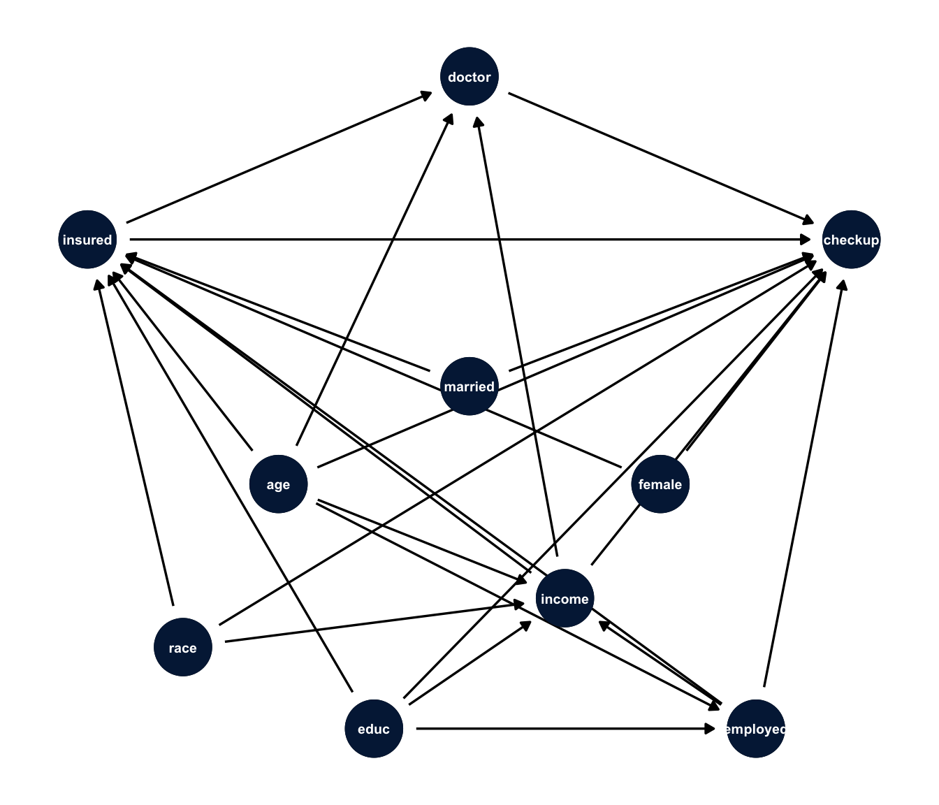
NoteCode explanation:
dagify()
dagify() takes formulas where the left side is a variable and the right side lists its direct causes, so doctor ~ insured + age + income means “insurance, age and income each have an arrow into having a regular doctor.” exposure and outcome mark the treatment and the outcome. coords places the nodes so the picture is readable; without it, ggdag() picks a layout at random. geom_dag_point() and geom_dag_text() redraw the nodes and labels in our colors.
What to adjust for
The DAG tells us which variables to adjust for, using the backdoor criterion: adjust for a set of variables that blocks every path from the treatment to the outcome that starts with an arrow into the treatment (a “backdoor” path), without adjusting for anything caused by the treatment. dagitty finds those sets for you.
adjustmentSets(dag)#> { age, educ, employed, female, income, married, race }The minimal set is the seven demographic and socioeconomic variables. Two things are not in it, and both matter.
- Mediators. Having a regular doctor is on the path from insurance to checkups. When the question is the total effect of insurance, as ours is, adjusting for it would remove part of the effect we’re trying to estimate, the part that works by giving people a doctor. So, for a total effect, don’t adjust for variables caused by the treatment. (Questions about direct effects, like “how much does insurance matter apart from getting people a doctor?”, are a different question, with their own methods and stronger assumptions.)
- Colliders. A collider is a variable caused by two others, like \(X \rightarrow C \leftarrow Y\). Two causes of a collider are independent until you condition on it; then they become associated. The classic example: if admission to a selective program depends on either talent or connections, then among the admitted, talent and connections are negatively correlated, even if they’re unrelated in the population (Elwert and Winship 2014). Adjusting for a collider, or selecting your sample on one, creates bias that wasn’t there. A surprising number of “controls” in published regressions are colliders.
collider <- dagify(C ~ X + Y, coords = list(x = c(X = 0, C = 1, Y = 2), y = c(X = 0, C = -1, Y = 0)))

ggdag(collider, text = FALSE, node_size = 12) +
  geom_dag_point(colour = utsa_cols("midnight"), size = 12) +
  geom_dag_text(colour = "white") +
  theme_dag()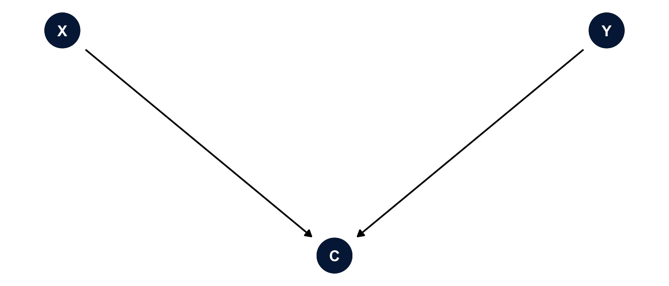
The DAG is only as good as your knowledge. If I’ve left out a confounder (like health status, which affects both insurance through Medicaid disability eligibility and checkups), no method below will fix it. Drawing the DAG doesn’t make the assumptions true, but it makes them visible, so readers can argue with them.
The data
The BRFSS asks how long it’s been since each respondent’s last routine checkup. I’ll use adults 18 to 64, since nearly everyone 65 and over has Medicare.
brfss <- get_mmsa() |>
  recode_mmsa() |>
  mutate(checkup = case_when(checkup1 == 1 ~ 1,               # within the past year
                             checkup1 %in% c(2:4, 8) ~ 0),    # longer ago, or never
         employed = case_when(employ1 %in% 1:2 ~ "Employed",
                              employ1 %in% 3:4 ~ "Unemployed",
                              employ1 %in% 5:6 ~ "Homemaker or student",
                              employ1 == 7 ~ "Retired",
                              employ1 == 8 ~ "Unable to work"),
         married = case_when(marital == 1 ~ 1, marital %in% 2:6 ~ 0),
         age = age80) |>
  filter(agec != "65+") |>
  select(checkup, insured, age, female, race_eth, educ, income, employed, married,
         mmsawt, ststr) |>
  drop_na() |>
  mutate(sw = mmsawt / mean(mmsawt))       # survey weight rescaled to average 1

des <- svydesign(ids = ~1, strata = ~ststr, weights = ~sw, data = brfss)
svyby(~checkup, ~insured, design = des, FUN = svymean)
#> insured checkup se
#> 0 0 0.4155586 0.010725826
#> 1 1 0.7720683 0.0026167439.6% of these adults are uninsured. The unadjusted difference in the share with a checkup in the past year is 35.7 percentage points. Some of that is confounding.
WarningThe timing problem
A causal claim needs the treatment to come before the outcome. These data don’t give us that. The BRFSS asks whether someone is insured now and whether they had a checkup in the past year. Someone insured today may have been uninsured at the time of their checkup, or may have gotten coverage because a checkup found a problem. So the example illustrates the methods, and the assumptions they need, but even with perfect adjustment it wouldn’t establish that insurance came first. A real study would use data that measure insurance before the outcome period, like a panel survey or administrative records. Keep this in mind for every estimate below.
Note
I dropped people with missing values on any of these variables, which is about a quarter of the sample, mostly because of income. A real analysis would use multiple imputation from week 9 first, and then do everything below within each imputed data set.
Propensity scores
The idea
With seven confounders, many of them categorical, there are thousands of combinations of \(X\), and we can’t compare insured and uninsured people within every one. Rosenbaum and Rubin (1983) showed that we don’t have to. The propensity score, \(e(X) = \Pr(\text{insured} \mid X)\), is a single number that summarizes the confounders, and if exchangeability holds given \(X\), it also holds given \(e(X)\). So we can balance the groups on the propensity score instead of on every combination of the confounders. Austin (2011) is a good practical introduction.
There are two main ways to use it.
- Matching pairs each uninsured person with an insured person who has a similar propensity score, throws away the insured people who aren’t anyone’s match, and compares the matched groups.
- Weighting keeps everyone and reweights the groups so that each looks like the target population. For the ATC, the uninsured keep a weight of 1, and each insured person gets a weight of \((1 - e)/e\), which makes the insured look like the uninsured. (For the ATE, everyone gets \(1/\Pr(\text{the treatment they got})\), and for the ATT, the insured keep 1 and the uninsured get \(e/(1 - e)\).)
I’ll do weighting with WeightIt first, then matching with MatchIt. They answer the same question, and both packages are written to work with cobalt for checking balance, so the workflow is the same: estimate, check balance, then estimate the effect.
Propensity scores with survey data
With survey data, there are two populations to think about: the population the survey represents, and the population of people the propensity weights describe. DuGoff et al. (2014) recommend fitting the propensity score model with the survey weights and then multiplying the propensity weights by the survey weights for the outcome analysis, so that the estimate describes the treatment effect in the survey’s target population. WeightIt does the first part with its s.weights argument.
f_ps <- insured ~ age + I(age^2) + female + race_eth + educ + income + employed + married

w_glm <- weightit(f_ps, data = brfss, method = "glm", estimand = "ATC", s.weights = "sw")
summary(w_glm)
#> Summary of weights
#>
#> ─ Weight ranges:
#>
#> Min Max
#> Treated 0. ╞══════════════════╡ 31.572
#> Control 0.004 ╞═══════════════════════════╡ 45.678
#>
#> ─ Units with the 5 most extreme weights by group:
#>
#> 59301 76908 45490 57065 59348
#> Treated 23.312 25.158 25.175 30.824 31.572
#> 45881 45441 45602 94400 45889
#> Control 35.606 36.263 38.035 38.88 45.678
#>
#> ─ Weight statistics:
#>
#> Coef of Var MAD Entropy # Zeros
#> Treated 4.694 1.302 1.745 0
#> Control 1.86 0.894 0.746 0
#>
#> ─ Effective Sample Sizes:
#>
#> Control Treated
#> Unweighted 2093.95 26044.37
#> Weighted 2093.95 4682.37
NoteCode explanation:
weightit()
- The formula is the propensity score model: the treatment on the left, the confounders on the right. Its job is balance, not prediction, so include what the DAG says and don’t worry about significance.
method = "glm"estimates the propensity score with a logit model, andestimand = "ATC"computes the ATC weights from it.s.weights = "sw"names the survey weight, which is used in fitting the propensity model and in the balance statistics. The weightsweightit()returns don’t include the survey weights; you multiply them in for the outcome model.summary()shows the range of the weights and the effective sample size (ESS), roughly how many unweighted observations the weighted sample is worth. Very large weights shrink the ESS, and they’re a warning that some people are carrying a lot of the estimate.
Checking balance
The point of the propensity score is to balance the confounders, so check whether it did. The usual measure is the standardized mean difference: the difference in means between groups divided by the standard deviation. A common rule is that it should be below 0.1 for every covariate after weighting.
love.plot(w_glm, thresholds = c(m = 0.1), abs = TRUE, binary = "std",
          colors = c(utsa_cols("orange")[[1]], utsa_cols("midnight")[[1]]),
          shapes = c("triangle", "circle"), var.order = "unadjusted",
          sample.names = c("Unweighted", "Weighted")) +
  theme(legend.position = "bottom")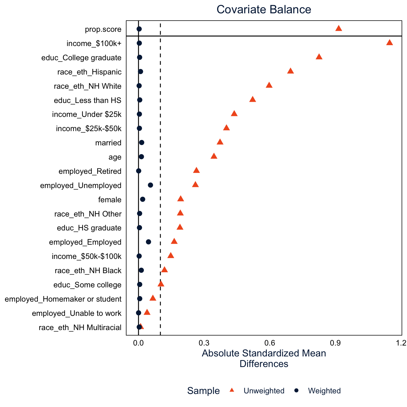
Before weighting, the insured and uninsured differ by more than 0.1 standard deviations on most of the confounders, by more than 0.5 on some, like income and Hispanic ethnicity. After weighting, every one is under 0.1. In the weighted data, insured and uninsured adults look alike on everything in the model. That’s the thing propensity scores can do that ordinary regression can’t: you can see whether the adjustment worked, before you look at the outcome.
Be precise about what “worked” means, though. Balance is about the measured covariates, and about the summaries you checked (here, means). A standardized difference below 0.1 says the groups have similar means on age, income and the rest. It says nothing about health status, motivation, or anything else we didn’t measure, so it doesn’t establish exchangeability. Good balance is necessary, not sufficient.
NoteCode explanation:
love.plot()
love.plot() from cobalt plots the standardized mean difference for every covariate, before and after adjustment. abs = TRUE plots absolute values, binary = "std" standardizes binary variables too, thresholds = c(m = 0.1) draws the 0.1 line, and var.order = "unadjusted" sorts the covariates by how unbalanced they were. bal.tab(w_glm) gives the same information as a table.
Estimating the effect
Now the outcome model. With balance achieved by the weights, the outcome model can be simple: checkup on insurance, with the propensity weights times the survey weights.
brfss$w_ps <- w_glm$weights * brfss$sw
des_ps <- svydesign(ids = ~1, strata = ~ststr, weights = ~w_ps, data = brfss)
fit_ps <- svyglm(checkup ~ insured, design = des_ps, family = quasibinomial)

atc_ps <- avg_comparisons(fit_ps, variables = "insured", wts = "(weights)")
atc_ps
#>
#> Estimate Std. Error z Pr(>|z|) S 2.5 % 97.5 %
#> 0.297 0.0128 23.2 <0.001 394.2 0.272 0.322
#>
#> Term: insured
#> Type: response
#> Comparison: 1 - 0
TipReading the result: a right and a wrong interpretation
Right: “If insured and uninsured adults are exchangeable given the measured characteristics, and setting aside the timing problem, weighting estimates that having insurance would raise the probability of a past-year checkup among the currently uninsured by 29.7 percentage points (95% CI 27.2 to 32.2).”
Wrong: “Insurance causes a 29.7 percentage point increase in checkups.” That states the causal conclusion without the assumptions it rests on. Weighting made the insured and uninsured similar on measured characteristics; it can’t establish that insurance came before the checkup or remove confounding from variables we didn’t measure. The calculation illustrates a method; the causal interpretation needs a separate argument.
Warning
The standard errors here treat the propensity weights as fixed, which isn’t quite right, because they were estimated. In practice, that usually makes them a little conservative for the ATE and ATC. For exact standard errors, use the glm_weightit() function in WeightIt, which accounts for the estimation of the weights (but not the survey strata), or bootstrap the whole procedure with replicate weights, as in week 7.
Matching
Nearest neighbor matching
Matching is the oldest and most intuitive way to use the propensity score (Stuart 2010). For the ATC, the uninsured are the group we want to learn about, so for each uninsured person we find the insured person whose propensity score is closest, and set the rest of the insured aside. If the matching works, the matched insured group looks like the uninsured group on all the measured confounders, and comparing their checkup rates is comparing like with like on those characteristics. An experiment would balance the unmeasured ones too; matching can’t.
MatchIt does the matching. Its main function, matchit(), uses the same formula as weightit(), and I’ll also set a caliper: a maximum distance allowed between the propensity scores of a matched pair. An uninsured person with no insured person within the caliper goes unmatched, instead of being paired with someone who isn’t really similar.
m_nn <- matchit(f_ps, data = brfss, method = "nearest", distance = "glm",
                estimand = "ATC", caliper = 0.2, s.weights = ~sw)
summary(m_nn, un = FALSE)
#>
#> Call:
#> matchit(formula = f_ps, data = brfss, method = "nearest", distance = "glm",
#> estimand = "ATC", s.weights = ~sw, caliper = 0.2)
#>
#> Summary of Balance for Matched Data:
#> Means Treated Means Control Std. Mean Diff.
#> distance 0.7590 0.7743 -0.0875
#> age 38.1743 37.9531 0.0186
#> I(age^2) 1603.3565 1583.6153 0.0206
#> female 0.4381 0.4292 0.0180
#> race_ethNH White 0.2633 0.2754 -0.0274
#> race_ethNH Black 0.0978 0.1127 -0.0481
#> race_ethNH Other 0.0497 0.0598 -0.0435
#> race_ethNH Multiracial 0.0246 0.0277 -0.0196
#> race_ethHispanic 0.5646 0.5243 0.0809
#> educLess than HS 0.2994 0.2753 0.0524
#> educHS graduate 0.3448 0.3257 0.0412
#> educSome college 0.2354 0.2561 -0.0482
#> educCollege graduate 0.1205 0.1429 -0.0653
#> incomeUnder $25k 0.3122 0.3118 0.0009
#> income$25k-$50k 0.3799 0.3703 0.0197
#> income$50k-$100k 0.2166 0.2174 -0.0020
#> income$100k+ 0.0913 0.1005 -0.0311
#> employedEmployed 0.6720 0.6685 0.0075
#> employedHomemaker or student 0.1226 0.1255 -0.0091
#> employedRetired 0.0140 0.0129 0.0107
#> employedUnable to work 0.0343 0.0476 -0.0636
#> employedUnemployed 0.1570 0.1455 0.0323
#> married 0.3322 0.3408 -0.0181
#> Var. Ratio eCDF Mean eCDF Max Std. Pair Dist.
#> distance 1.0082 0.0213 0.0641 0.0084
#> age 1.0202 0.0065 0.0226 0.3386
#> I(age^2) 1.0216 0.0065 0.0226 0.3311
#> female . 0.0089 0.0089 0.2870
#> race_ethNH White . 0.0121 0.0121 0.1602
#> race_ethNH Black . 0.0149 0.0149 0.1392
#> race_ethNH Other . 0.0101 0.0101 0.1368
#> race_ethNH Multiracial . 0.0032 0.0032 0.1611
#> race_ethHispanic . 0.0403 0.0403 0.1705
#> educLess than HS . 0.0241 0.0241 0.1812
#> educHS graduate . 0.0191 0.0191 0.2294
#> educSome college . 0.0208 0.0208 0.1595
#> educCollege graduate . 0.0224 0.0224 0.1411
#> incomeUnder $25k . 0.0004 0.0004 0.3144
#> income$25k-$50k . 0.0096 0.0096 0.2958
#> income$50k-$100k . 0.0008 0.0008 0.1335
#> income$100k+ . 0.0092 0.0092 0.0600
#> employedEmployed . 0.0035 0.0035 0.3226
#> employedHomemaker or student . 0.0030 0.0030 0.2288
#> employedRetired . 0.0012 0.0012 0.0797
#> employedUnable to work . 0.0133 0.0133 0.1687
#> employedUnemployed . 0.0115 0.0115 0.3420
#> married . 0.0086 0.0086 0.2990
#>
#> Sample Sizes:
#> Control Treated
#> All (ESS) 2093.95 26044.37
#> All 9339. 107858.
#> Matched (ESS) 2064.83 2197.03
#> Matched 9091. 9091.
#> Unmatched 248. 98767.
#> Discarded 0. 0.
NoteCode explanation:
matchit() and summary()
- The formula is the propensity score model, the same
f_pswe gaveweightit(). method = "nearest"is nearest neighbor matching, anddistance = "glm"estimates the propensity score with a logit model, the same model asmethod = "glm"inweightit(). The propensity score is called the distance inMatchIt, because it’s what the matching measures closeness on.estimand = "ATC"tellsmatchit()which group to find matches for.MatchItcalls the group withinsured == 1the “treated” group and the group withinsured == 0the “control” group, so with the ATC every uninsured person (control) gets an insured (treated) match. With the default,estimand = "ATT", it would go the other way.caliper = 0.2allows matches only within 0.2 standard deviations of the propensity score. Smaller calipers give closer matches but leave more people unmatched.- By default, each uninsured person gets one match (
ratio = 1), and an insured person can be used only once (replace = FALSE). I’ll change both below. s.weights = ~swnames the survey weight, as inweightit(), except thatmatchit()wants it as a one-sided formula, with a~. It’s used to fit the propensity score model and in the balance statistics, and, unlike inWeightIt, it’s also included in the weightsmatchit()returns (more on that below).summary()prints a balance table and a table of sample sizes.un = FALSEleaves out the balance before matching, which we’ll see in the plot below. The Std. Mean Diff. column is the standardized mean difference from the weighting section, and Var. Ratio is the ratio of the variances in the two groups, which should be close to 1 for continuous variables like age. The eCDF columns compare the whole distributions (0 means identical), and Std. Pair Dist. is how far apart the two people in a pair are, on average. The sample size table shows how many people were matched and unmatched in each group, and the effective sample size (ESS).
NoteReference: the main
matchit() arguments
| Argument | What it does |
|---|---|
formula |
Treatment on the left, confounders on the right. This is the propensity score model, or for method = "cem" and method = "exact", the variables to match on. |
data |
The data frame that holds the variables. |
method |
How to match. "nearest" (nearest neighbor, the default), "optimal" and "full" (both need the optmatch package), "cem" (coarsened exact matching), "exact", and "subclass" (subclassification on the propensity score). |
distance |
How to measure closeness. "glm" (the default) is a logit propensity score. Others include "gbm" and "randomforest" for machine learning propensity scores, and "mahalanobis" to match on the covariates directly. |
link |
With distance = "glm", link = "linear.logit" matches on the logit of the propensity score instead of the probability. |
estimand |
"ATT" (the default) finds matches for the treated, "ATC" finds matches for the controls. Nearest neighbor matching can’t estimate the ATE, but "full", "cem" and "subclass" can. |
ratio |
How many matches each focal person gets. The default is 1. |
replace |
Whether a person can be used as a match more than once. The default is FALSE. |
caliper |
The largest allowed distance in a pair, in standard deviations of the distance measure. The common rule of 0.2 (Austin 2011) is for the logit of the propensity score, so pair it with link = "linear.logit" if you want to follow that rule exactly. |
exact |
A one-sided formula, like ~ race_eth, for variables that have to match exactly. Matching on the propensity score then happens within each group. |
s.weights |
The survey weights, as a one-sided formula. |
?matchit lists the rest, and the package’s “Matching Methods” vignette explains when to use each method.
The distance that matchit() estimated is an ordinary logit model of being insured, the kind of model we fit in week 3. You can fit it yourself with svyglm() and get the same propensity scores.
ps_mod <- svyglm(f_ps, design = des, family = quasibinomial)
summary(ps_mod)
#>
#> Call:
#> svyglm(formula = f_ps, design = des, family = quasibinomial)
#>
#> Survey design:
#> svydesign(ids = ~1, strata = ~ststr, weights = ~sw, data = brfss)
#>
#> Coefficients:
#> Estimate Std. Error t value Pr(>|t|)
#> (Intercept) 2.292032 0.271897 8.430 < 2e-16 ***
#> age -0.105754 0.013817 -7.654 1.96e-14 ***
#> I(age^2) 0.001489 0.000171 8.705 < 2e-16 ***
#> female 0.482792 0.052425 9.209 < 2e-16 ***
#> race_ethNH Black 0.041672 0.092197 0.452 0.65127
#> race_ethNH Other 0.006252 0.104959 0.060 0.95250
#> race_ethNH Multiracial -0.348443 0.133337 -2.613 0.00897 **
#> race_ethHispanic -0.859103 0.056369 -15.241 < 2e-16 ***
#> educHS graduate 0.799761 0.074317 10.761 < 2e-16 ***
#> educSome college 1.033076 0.080079 12.901 < 2e-16 ***
#> educCollege graduate 1.541002 0.090154 17.093 < 2e-16 ***
#> income$25k-$50k 0.063855 0.067748 0.943 0.34592
#> income$50k-$100k 0.746596 0.081721 9.136 < 2e-16 ***
#> income$100k+ 1.706827 0.109418 15.599 < 2e-16 ***
#> employedHomemaker or student 0.065566 0.086758 0.756 0.44981
#> employedRetired 0.670366 0.206316 3.249 0.00116 **
#> employedUnable to work 0.816060 0.150608 5.418 6.02e-08 ***
#> employedUnemployed -0.429436 0.085563 -5.019 5.20e-07 ***
#> married 0.178308 0.060548 2.945 0.00323 **
#> ---
#> Signif. codes: 0 '***' 0.001 '**' 0.01 '*' 0.05 '.' 0.1 ' ' 1
#>
#> (Dispersion parameter for quasibinomial family taken to be 0.9623289)
#>
#> Number of Fisher Scoring iterations: 6all.equal(fitted(ps_mod), m_nn$distance, check.attributes = FALSE)#> [1] TRUEThe coefficients tell us who is insured: insurance rises with education and income, women are more likely to be insured than men, unemployed adults are less likely than employed adults, and Hispanic adults are much less likely to be insured than NH White adults with the same education and income. fitted() gives each person’s predicted probability of being insured, and all.equal() confirms these are the same numbers matchit() used (check.attributes = FALSE tells it to compare only the values, not the names attached to them).
Tip
You’ll sometimes see propensity score models judged by how well they predict treatment, with a confusion matrix or an AUC. That’s the wrong yardstick. A propensity model that predicts treatment perfectly is actually bad news, because it means there are people with no comparable counterparts in the other group. The propensity score’s job is balance, so judge it by the balance it produces.
9,091 of the 9,339 uninsured adults found a match within the caliper, and 248 didn’t. Those 248 are people with propensity scores that no insured person has: they look so much like the typical uninsured person that there’s no insured person like them. Dropping them changes the estimand a little. We’re now estimating the ATC for the uninsured people who have a comparable insured person, which is worth saying in a paper. It’s a positivity problem showing up in the data, and matching makes it visible.
Checking balance after matching
cobalt works on matchit() output just as it does on weightit() output, so the love plot from the weighting section works without changes.
love.plot(m_nn, thresholds = c(m = 0.1), abs = TRUE, binary = "std",
          colors = c(utsa_cols("orange")[[1]], utsa_cols("midnight")[[1]]),
          shapes = c("triangle", "circle"), var.order = "unadjusted",
          sample.names = c("Unmatched", "Matched")) +
  theme(legend.position = "bottom")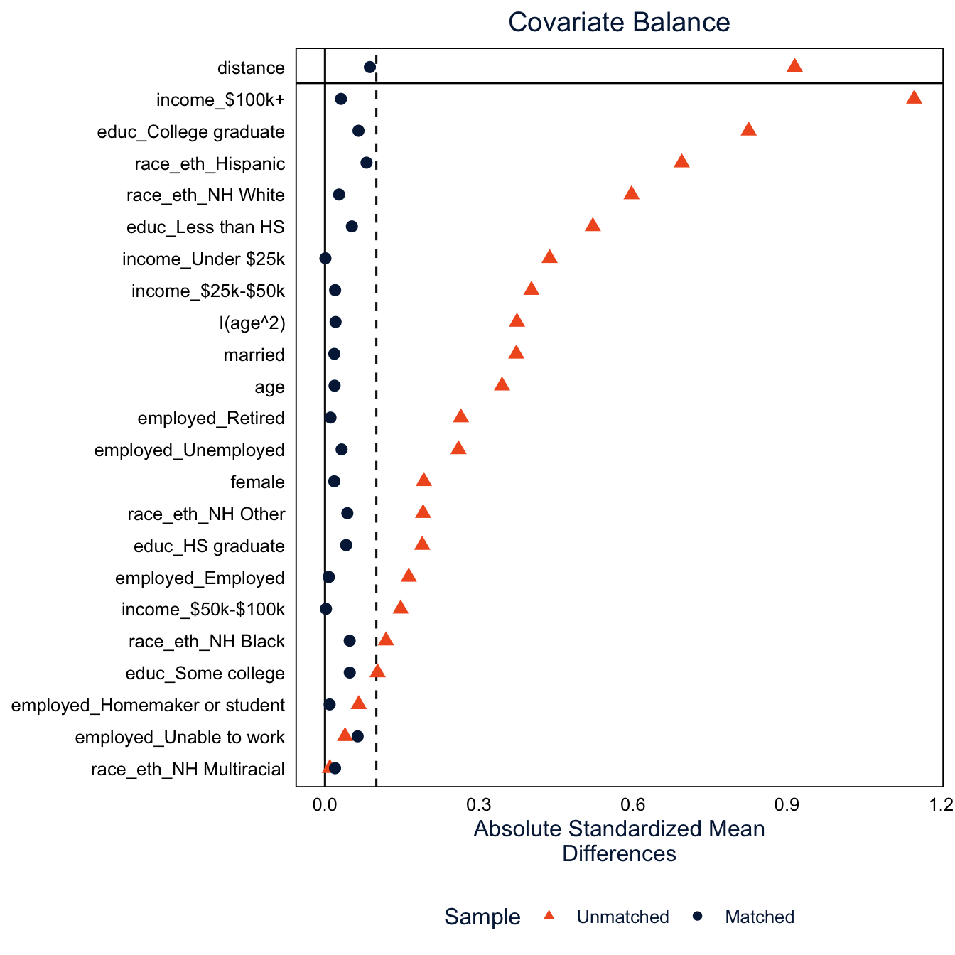
After matching, every covariate has a standardized mean difference under 0.1. The balance is a bit less exact than with weighting, because each uninsured person gets one specific match, and the matches aren’t perfect. The “distance” row at the top is the propensity score itself.
It’s also worth looking at the whole distribution of the propensity score in each group, not only its mean. This is how we check common support: whether the two groups cover the same range of propensity scores. It’s the most direct way to see positivity.
bal.plot(m_nn, var.name = "distance", which = "both", type = "histogram", mirror = TRUE,
         colors = c(utsa_cols("midnight")[[1]], utsa_cols("orange")[[1]]),
         sample.names = c("Unmatched", "Matched")) +
  scale_y_continuous(labels = abs) +
  labs(x = "Propensity score", fill = "Insured", title = NULL) +
  theme(legend.position = "bottom")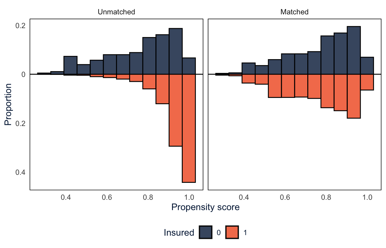
NoteCode explanation:
bal.plot()
bal.plot()fromcobaltplots the distribution of one variable in each group.var.name = "distance"picks the propensity score (any covariate in the model works too, likevar.name = "age"), andwhich = "both"draws it before and after matching side by side.type = "histogram", mirror = TRUEdraws a mirror histogram: one group’s histogram above the line and the other’s flipped below it, so you can compare them bar by bar.type = "density"would draw overlapping density curves instead.- The bars below the line are proportions shown as negative numbers, so
scale_y_continuous(labels = abs)labels the axis with their absolute values.abs()is the absolute value function, passed tolabelswithout parentheses so thatggplotcan apply it to each label. - Like
love.plot(),bal.plot()returns aggplot, solabs()andtheme()work on it.
Before matching (left), most insured adults have propensity scores above 0.9, while the uninsured are spread out, with a lot of them below 0.7. After matching (right), the two histograms are mirror images: the matched insured people are the ones who looked, before the fact, like they might well have been uninsured.
Estimating the effect
match.data() returns the matched sample: the uninsured people who were matched and their insured matches, with everyone else dropped. Sorting it by subclass puts each pair together, so you can see who was matched to whom.
md_nn <- match.data(m_nn)

md_nn |>
  arrange(subclass) |>
  select(subclass, insured, age, female, race_eth, educ, income, distance, sw, weights) |>
  head(6)
#> # A tibble: 6 × 10
#> subclass insured age female race_eth educ income distance sw weights
#> <fct> <dbl> <dbl> <dbl> <fct> <fct> <fct> <dbl> <dbl> <dbl>
#> 1 1 0 63 1 NH White HS grad… $25k-… 0.976 0.0320 0.0320
#> 2 1 1 63 1 NH White HS grad… $25k-… 0.976 0.159 0.159
#> 3 2 0 52 1 NH Other College… $50k-… 0.978 0.0564 0.0564
#> 4 2 1 52 1 NH Other College… $50k-… 0.978 3.35 3.35
#> 5 3 0 49 0 Hispanic HS grad… Under… 0.651 0.0722 0.0722
#> 6 3 1 49 0 Hispanic HS grad… Under… 0.651 0.161 0.161
NoteCode explanation:
match.data()
match.data()keeps only the matched people and adds three columns.distanceis each person’s propensity score.subclassidentifies the matched pairs: an uninsured person and their insured match have the same value.weightsis the matching weight.- With 1:1 matching without replacement, everyone in a pair would have a matching weight of 1, but because we gave
matchit()the survey weights,weightsalready includes the survey weight. That’s why theweightscolumn equalsswhere. So below, we useweightsdirectly, for the averages and in the survey design. This is different fromWeightIt, where we had to multiply the propensity weights byswourselves. Multiplyingmatch.data()’s weights byswagain would count the survey weights twice. arrange(subclass)sorts the rows so the people in each pair are next to each other.
With this many insured people to choose from, many uninsured people find an insured match who is the same on every covariate, like the first three pairs here. That won’t always happen: two people can have about the same propensity score while differing on a covariate, if they also differ on another one in the opposite direction. Matching makes the groups alike on average, not necessarily every pair, which is why we check balance across the whole matched sample.
Look at the survey weights, though. In the second pair, the insured person’s survey weight is about 60 times the uninsured person’s. Each person keeps their own survey weight after matching, so the two halves of a pair don’t count the same in the weighted analysis. We’ll come back to this.
With one match per person and no replacement, the effect is just the difference between the share with a checkup in the matched insured and uninsured groups, using the weights.
md_nn |>
  group_by(insured) |>
  summarise(checkup = weighted.mean(checkup, weights))
#> # A tibble: 2 × 2
#> insured checkup
#> <dbl> <dbl>
#> 1 0 0.424
#> 2 1 0.723weighted.mean() is an average that counts each person by their weight. The average of a 0/1 variable is a share, so this is the weighted share with a checkup in each group.
The model below gives the same difference, along with a standard error that accounts for the survey design.
des_nn <- svydesign(ids = ~1, strata = ~ststr, weights = ~weights, data = md_nn)
fit_nn <- svyglm(checkup ~ insured, design = des_nn, family = quasibinomial)

atc_nn <- avg_comparisons(fit_nn, variables = "insured", wts = "(weights)")
atc_nn
#>
#> Estimate Std. Error z Pr(>|z|) S 2.5 % 97.5 %
#> 0.299 0.0144 20.8 <0.001 317.6 0.271 0.327
#>
#> Term: insured
#> Type: response
#> Comparison: 1 - 0The estimate is the difference between the two weighted shares above. The design and the model are the same as in the weighting section, except that the weights come from match.data().
Warning
The MatchIt documentation recommends standard errors that account for the matched pairs, since the two people in a pair were chosen to be alike. You can do that by using ids = ~subclass in svydesign(), but then you can’t also use the survey strata. Here, the standard error is about the same either way, but with smaller samples or stronger matching it may not be. The “Estimating Effects After Matching” vignette that comes with MatchIt covers this in detail.
Matching choices (optional)
Nearest neighbor 1:1 matching without replacement is the default, but there are other choices to make, and matching is usually a process of trying a few, checking balance each time, and improving. Four choices matter here.
- Ratio. With
ratio = 3, each uninsured person gets their three closest insured matches. More matches means a bigger sample and smaller standard errors, but the second and third matches are further away than the first, so balance can get worse. - Replacement. With
replace = TRUE, an insured person can be the match for more than one uninsured person. Every uninsured person gets their closest match, which should mean closer matches, but an insured person who is used many times carries a lot of weight, which increases the standard error. - Exact matching. If one covariate is especially important, or still unbalanced after matching,
exactforces every pair to be the same on it, and matches on the propensity score only within those groups. - The method. Nearest neighbor matching on the propensity score is one method of several. Coarsened exact matching (CEM) doesn’t use a propensity score at all. It cuts continuous variables like age into bins, then matches people exactly on every variable, so an uninsured person is matched to every insured person in the same “cell”: same age group, sex, race and ethnicity, education, income, employment and marital status. Anyone in a cell with no one from the other group is dropped.
# 3:1 matching without replacement
m_k3 <- matchit(f_ps, data = brfss, method = "nearest", estimand = "ATC",
                ratio = 3, caliper = 0.2, s.weights = ~sw)

# 1:1 matching with replacement
m_rep <- matchit(f_ps, data = brfss, method = "nearest", estimand = "ATC",
                 replace = TRUE, s.weights = ~sw)

# 1:1 matching with replacement, exactly on race and ethnicity
m_rep_ex <- matchit(f_ps, data = brfss, method = "nearest", estimand = "ATC",
                    replace = TRUE, exact = ~ race_eth, s.weights = ~sw)

# coarsened exact matching
m_cem <- matchit(insured ~ age + female + race_eth + educ + income + employed + married,
                 data = brfss, method = "cem", estimand = "ATC", s.weights = ~sw)
NoteCode explanation:
exact and method = "cem"
exact = ~ race_ethsplits the data by race and ethnicity and does the nearest neighbor matching separately within each group, so a Hispanic uninsured person can only be matched to a Hispanic insured person. You can list more than one variable, likeexact = ~ race_eth + female, but every variable you add makes the groups smaller and the matches harder to find.method = "cem"does coarsened exact matching. The formula lists the variables to match on, not a propensity score model, which is why it doesn’t haveI(age^2): once age is cut into bins, the square of age adds nothing. Categorical variables are matched exactly as they are, andmatchit()picks the bins for continuous variables (you can set your own with thecutpointsargument).- CEM returns weights instead of pairs. Within each cell, the insured people are weighted so they count as much as the uninsured people in that cell, using the survey weights.
To compare all the versions, I’ll fit the same outcome model to each one and put the results in a table.
# fit the outcome model to a matched sample
match_effect <- function(m) {
  md <- match.data(m)
  fit <- svyglm(checkup ~ insured, family = quasibinomial,
                design = svydesign(ids = ~1, strata = ~ststr, weights = ~weights, data = md))
  avg_comparisons(fit, variables = "insured", wts = "(weights)")
}

# the largest standardized mean difference after matching
max_smd <- function(m) {
  bal <- bal.tab(m, binary = "std")$Balance
  bal <- bal[rownames(bal) != "distance", ]
  max(abs(bal$Diff.Adj))
}

matches <- list("1:1" = m_nn, "3:1" = m_k3, "1:1, replacement" = m_rep,
                "1:1, replacement, exact on race and ethnicity" = m_rep_ex,
                "Coarsened exact matching" = m_cem)
effects <- map(matches, match_effect)

match_tab <- tibble(
  matching = names(matches),
  uninsured_matched = map_dbl(matches, \(m) sum(m$weights > 0 & brfss$insured == 0)),
  insured_used = map_dbl(matches, \(m) sum(m$weights > 0 & brfss$insured == 1)),
  max_smd = map_dbl(matches, max_smd),
  estimate = map_dbl(effects, "estimate"),
  se = map_dbl(effects, "std.error"))
knitr::kable(match_tab, digits = 3)| matching | uninsured_matched | insured_used | max_smd | estimate | se |
|---|---|---|---|---|---|
| 1:1 | 9091 | 9091 | 0.081 | 0.299 | 0.014 |
| 3:1 | 9091 | 23153 | 0.065 | 0.287 | 0.013 |
| 1:1, replacement | 9339 | 7423 | 0.119 | 0.307 | 0.018 |
| 1:1, replacement, exact on race and ethnicity | 9339 | 7414 | 0.121 | 0.298 | 0.018 |
| Coarsened exact matching | 8637 | 73723 | 0.000 | 0.284 | 0.014 |
atc_k3 <- effects[["3:1"]]
NoteCode explanation:
match_effect(), max_smd() and map_dbl()
match_effect()is a function we write ourselves, likemymean()in week 1. It wraps the three steps from the last section (match.data(),svyglm(),avg_comparisons()) into one function, so we can run them on each matched result without copying the code.function(m)says it takes one input, calledminside the function, and the last line is what it returns.max_smd()takes the balance table frombal.tab(), the table version of the love plot, and returns the largest absolute standardized mean difference after matching. The row names of the table are the covariates, andrownames(bal) != "distance"drops the propensity score row, which CEM doesn’t have.Diff.Adjis the column of differences after matching.matchesis a named list of the five matched results.map(), from week 2, runsmatch_effect()on each one and returns a list of results.map_dbl()does the same but returns a plain vector of numbers, which is what a table column needs.\(m) sum(m$weights > 0 & brfss$insured == 0)is a function written on the fly, as in week 2.m$weights > 0isTRUEfor everyone who was matched, so this counts the matched uninsured people.map_dbl(effects, "estimate")uses a shortcut: given a name instead of a function,map_dbl()pulls out the element with that name from each result, so this is the same asmap_dbl(effects, \(e) e$estimate).effects[["3:1"]]pulls one element out of the list by name, to use in the comparison with the other methods below.
The 3:1 match uses about three times as many insured people as the 1:1 match, has a smaller standard error, and in this case balances a little better too, since there are plenty of insured people close to each uninsured person. Matching with replacement uses the fewest insured people, since some are used over and over, and has the largest standard error. It’s also the one that misses the balance goal: its largest standardized mean difference is 0.12, for Hispanic ethnicity.
Matching exactly on race and ethnicity should fix that, since now every pair has the same race and ethnicity. But the largest standardized mean difference is still 0.12, and it’s still for Hispanic ethnicity. The matching isn’t the problem; the survey weights are. As we saw in the matched pairs, each person keeps their own survey weight, so in the weighted analysis the insured half of a pair can count far more, or far less, than the uninsured half. Matching with replacement makes this worse, because an insured person with a large survey weight can be used again and again. The callout below shows one fix.
Coarsened exact matching balances every covariate almost perfectly, because it matches exactly within cells and the weights account for the survey weights within each cell. The cost is that 702 uninsured people are in cells with no insured people and get dropped, more than with the caliper, so its estimand moves further from the ATC for all the uninsured. With seven variables, there are a lot of cells, and with more variables CEM drops more and more people. That’s the problem the propensity score was invented to solve.
Here, I’d go with the 3:1 match, which balances well and keeps nearly all the uninsured, with CEM as a check. The estimates are all similar, which is reassuring. MatchIt has other methods too, including optimal matching and full matching, which need the optmatch package. Its “Matching Methods” vignette compares them.
WarningMatching and survey weights
MatchIt keeps each person’s own survey weight, which follows the approach of DuGoff et al. (2014). Austin et al. (2018) compared several ways of combining matching with survey weights, and found that a different approach worked better: give each matched person the survey weight of the person they were matched to. For the ATC, each insured match gets the survey weight of their uninsured partner. Then the two halves of every pair count equally, and the weighted matched sample represents the uninsured population.
MatchIt doesn’t do this for you, but get_matches() returns the pairs, and you can assign the weights yourself. Here it is for 1:1 matching with replacement.
gm <- get_matches(m_rep, data = brfss) |>
  group_by(subclass) |>
  mutate(w_pair = sw[insured == 0]) |>
  ungroup()

bal_pair <- bal.tab(f_ps, data = gm, weights = "w_pair", estimand = "ATC",
                    binary = "std", un = FALSE)
max(abs(bal_pair$Balance$Diff.Adj))
#> [1] 0.06030036fit_pair <- svyglm(checkup ~ insured, family = quasibinomial,
design = svydesign(ids = ~1, strata = ~ststr, weights = ~w_pair, data = gm))
avg_comparisons(fit_pair, variables = "insured", wts = "(weights)")#>
#> Estimate Std. Error z Pr(>|z|) S 2.5 % 97.5 %
#> 0.294 0.0148 19.9 <0.001 289.4 0.265 0.322
#>
#> Term: insured
#> Type: response
#> Comparison: 1 - 0get_matches()is likematch.data()(it needs the original data passed to it), but it returns one row per person per pair. With replacement, an insured person used as the match for five uninsured people appears five times, once in each pair.- Within each pair (
group_by(subclass)),sw[insured == 0]is the uninsured person’s survey weight, andmutate()gives it to both people in the pair. bal.tab()can check balance for any set of weights, not justmatchit()andweightit()results: give it the propensity score formula, the data and the name of the weight column.
With pair weights, the largest standardized mean difference drops from 0.12 to 0.06, the standard error shrinks, and the estimate barely changes. The standard error treats the duplicated rows as separate people, which isn’t quite right. For a careful analysis, cluster on the person’s id or bootstrap.
Tip
Like the propensity score model, the matching method is chosen by looking at balance, not at the outcome. Try different specifications, keep the one that balances best with the sample you can live with, and only then fit the outcome model. If you look at the estimate while you’re choosing, it’s easy to talk yourself into the specification that gives the answer you hoped for.
Other ways to get there (optional)
Logit propensity weights and nearest neighbor matching are two choices among many. Entropy balancing (Hainmueller 2012) skips the propensity model and finds weights that make the means of the covariates exactly equal across groups, while keeping the weights as even as possible. And plain regression adjustment, followed by averaging the predicted difference over the uninsured (like the average marginal effects from week 3), estimates the same ATC under different assumptions.
# entropy balancing
w_eb <- weightit(f_ps, data = brfss, method = "ebal", estimand = "ATC", s.weights = "sw")
brfss$w_eb <- w_eb$weights * brfss$sw
fit_eb <- svyglm(checkup ~ insured, family = quasibinomial,
                 design = svydesign(ids = ~1, strata = ~ststr, weights = ~w_eb, data = brfss))
atc_eb <- avg_comparisons(fit_eb, variables = "insured", wts = "(weights)")

# regression adjustment, averaged over the uninsured
fit_reg <- svyglm(update(f_ps, checkup ~ insured + .), design = des, family = quasibinomial)
atc_reg <- avg_comparisons(fit_reg, variables = "insured",
                           newdata = filter(brfss, insured == 0), wts = "sw")

results <- tibble(method = c("Unadjusted", "Regression adjustment", "Propensity score weights",
                             "Entropy balancing", "3:1 nearest neighbor matching"),
                  estimate = c(naive$estimate, atc_reg$estimate, atc_ps$estimate,
                               atc_eb$estimate, atc_k3$estimate),
                  se = c(naive$std.error, atc_reg$std.error, atc_ps$std.error,
                         atc_eb$std.error, atc_k3$std.error))
knitr::kable(results, digits = 3)| method | estimate | se |
|---|---|---|
| Unadjusted | 0.357 | 0.011 |
| Regression adjustment | 0.305 | 0.011 |
| Propensity score weights | 0.297 | 0.013 |
| Entropy balancing | 0.296 | 0.013 |
| 3:1 nearest neighbor matching | 0.287 | 0.013 |
NoteCode explanation:
update()
update(f_ps, checkup ~ insured + .) builds a new formula from an old one. The . on the right stands for everything that was on the right of f_ps, so this is checkup on insurance plus all the confounders. It saves retyping the list, and it guarantees the outcome model adjusts for the same variables as the propensity model.
results |>
  mutate(method = fct_rev(fct_inorder(method))) |>
  ggplot(aes(x = estimate, y = method)) +
  geom_pointrange(aes(xmin = estimate - 1.96 * se, xmax = estimate + 1.96 * se),
                  colour = utsa_cols("midnight")) +
  scale_x_continuous(labels = scales::label_percent()) +
  labs(x = "Difference in probability of a checkup", y = NULL)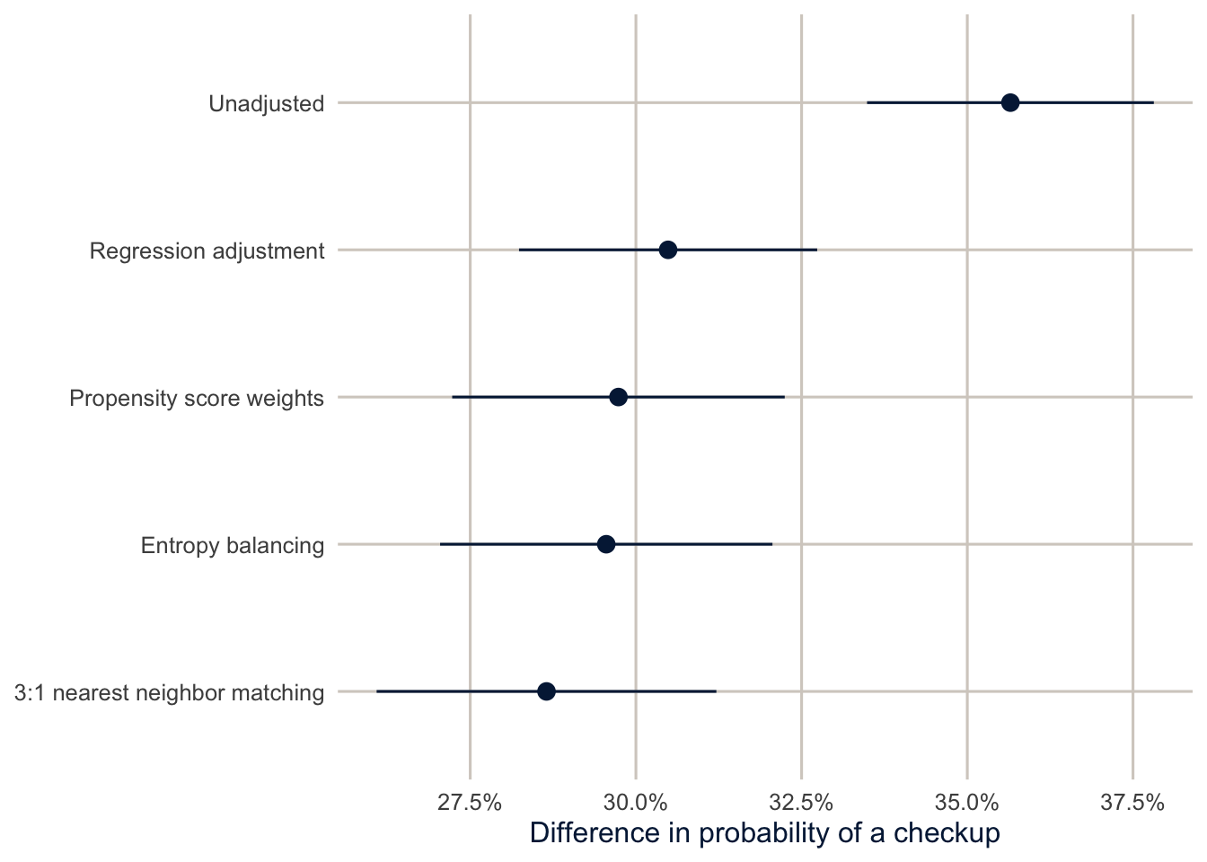
Regression adjustment, the two weighting methods and matching land close together, between 28.7 and 30.5 percentage points, compared with an unadjusted difference of 35.7. Adjusting for the confounders reduced the estimate a bit, but most of the gap survives. Matching is about as precise as weighting, even though it sets aside most of the insured sample, because the uninsured, not the insured, are the scarce group, and matching keeps all of them who have a comparable insured person. When very different methods agree, that’s reassuring, but remember that they all rely on the same assumption: no unmeasured confounding. They differ in how they adjust for the confounders, not in which confounders they adjust for.
How wrong could we be?
The biggest threat to this estimate is something we didn’t measure. Health is the obvious candidate: sicker people might be both more likely to get coverage (through disability-related Medicaid, for example) and more likely to see a doctor. VanderWeele and Ding (2017) proposed the E-value to put a number on how worried to be. It’s the minimum strength of association, on the risk ratio scale, that an unmeasured confounder would need to have with both the treatment and the outcome, beyond the measured confounders, to fully explain away the observed effect.
rr_ps <- avg_comparisons(fit_ps, variables = "insured", wts = "(weights)", comparison = "ratio")
ev <- evalues.RR(est = rr_ps$estimate, lo = rr_ps$conf.low, hi = rr_ps$conf.high)
ev
#> point lower upper
#> RR 1.715582 1.622764 1.808401
#> E-values 2.823572 2.628050 NAThe risk ratio is 1.72: insurance makes a past-year checkup about 1.7 times as likely for the uninsured. The E-value is 2.82. To explain the whole effect, an unmeasured confounder would need to make people 2.8 times as likely to be insured and 2.8 times as likely to get a checkup, after accounting for age, income, education and the rest. For the confidence interval to include no effect, it would need associations of 2.6. Those are strong associations, stronger than most of the measured confounders have. So unmeasured confounding alone would have to be quite strong to explain the result away.
Notice how narrow that statement is. The E-value answers one question, about an unmeasured confounder of a given strength. It says nothing about the timing problem (insurance measured now, checkups over the past year), about who is in the sample, about errors in how insurance or checkups were reported, or about whether “insured” is one well-defined treatment. Those are separate threats, and each needs its own argument. A fair summary of this example is: under the stated assumptions, the methods agree on an increase of about this size, and the result is robust to moderate unmeasured confounding, but the data can’t establish that insurance preceded the checkup.
Tip
Sensitivity analyses like this don’t prove anything. They translate “there might be unmeasured confounding” into a specific question that readers can think about: is there plausibly a confounder that strong? That’s a much better conversation than either ignoring the problem or giving up.
Summary
A causal effect compares potential outcomes that we can never see together, so we estimate averages, like the ATE, ATT or ATC, and need assumptions to do it: conditional exchangeability and positivity. A DAG makes the assumptions explicit and tells you what to adjust for, and what not to: for a total effect, not mediators, and never colliders. Propensity scores summarize the confounders in one number, and weighting or matching on them lets you check balance before looking at the outcome. Matching with MatchIt builds a comparison group of people who look like the group you care about, and it makes positivity problems visible as people who can’t be matched. With survey data, use the survey weights in the propensity model and in the outcome model: WeightIt leaves them out of its weights, so you multiply them in, and MatchIt’s match.data() already includes them. Different adjustment methods should give similar answers if the model is reasonable, but they all share the assumption of no unmeasured confounding, and an E-value tells you how strong a confounder would have to be to change your conclusion.
Homework 14
Due: April 29, before class.
Which version to do. If you’re in DEM 7283, do the version with your own survey data. If you’re in DEM 5283, do either version, and say at the top of your homework which one you did. If your survey can’t support this week’s method, do the version with my data and say so.
Purpose. Practice stating a causal question and its assumptions, estimating an effect with propensity scores, and being clear about what the analysis can and can’t establish.
A satisfactory answer defines the causal question before estimating anything; states the assumptions the estimate needs; reports balance and overlap; and explains what those checks don’t prove, including the timing limitation of these data.
With your own survey data
Use the full survey design for every estimate unless a step says otherwise, and report each estimate with a standard error or confidence interval.
- Choose a binary exposure (treatment) and an outcome in your data, and state a causal question about them. Define the target population and whether you want the average treatment effect (ATE) or the average treatment effect on the treated (ATT).
- Draw a DAG for your question with
dagittyandggdag.- Include the confounders you think matter, and at least one mediator or collider if your question has one.
- Find a minimal adjustment set. Which variables should you not adjust for, and why?
- Which important confounders aren’t measured in your data?
- Estimate propensity scores for the exposure with the variables in your adjustment set, and the survey weights, using
WeightIt.- Plot the distribution of propensity scores for the exposed and unexposed groups. Is there good overlap?
- Check balance before and after weighting with
cobalt, and show a Love plot. Is balance acceptable?
- Estimate the effect of the exposure using the combined propensity score and survey weights, and report it on the scale of the outcome (for example, in percentage points with
avg_comparisons()) with a confidence interval. - Compare it with the estimate from an ordinary survey-weighted regression with the same covariates. Are they similar?
- Calculate an E-value for your estimate, and interpret it. How strong would an unmeasured confounder need to be to explain away your result? Is that plausible for the confounders you named in step 2?
- In a paragraph, state the assumptions your estimate depends on (exchangeability, positivity, consistency) and how believable each one is here.
With my data
What is provided. The BRFSS analysis data brfss, the propensity score formula f_ps, the weights w_glm and the matched data from this chapter.
1. In your own words, define the causal question this chapter estimates: the treatment, outcome, eligible population, follow-up period and causal contrast. Draw a DAG for it (you can adapt the one in this chapter) and state the three assumptions the estimate needs, in plain language. Using the propensity score weights, show the overlap of the propensity scores and the balance of the covariates, and explain in two or three sentences why good balance and overlap don’t prove the estimate is causal. Finally, explain the timing limitation of using current insurance and a past-year checkup.
# YOUR CODE HERE2. Add doctor (having a personal doctor, from persdoc3: codes 1 and 2 are yes, 3 is no) to the propensity score model and redo the weighting. What happens to the estimate, and why is this the wrong thing to do?
# YOUR CODE HERE3. Estimate the ATT instead of the ATC (the effect of insurance for the people who have it). How do the weights, the effective sample size and the estimate change? Which estimand would you report to a state legislature considering a Medicaid expansion?
# YOUR CODE HEREOne solution for exercise 3
w_att <- weightit(f_ps, data = brfss, method = "glm", estimand = "ATT", s.weights = "sw")
summary(w_att)

brfss$w_att <- w_att$weights * brfss$sw
fit_att <- svyglm(checkup ~ insured, family = quasibinomial,
                  design = svydesign(ids = ~1, strata = ~ststr, weights = ~w_att, data = brfss))
avg_comparisons(fit_att, variables = "insured", wts = "(weights)")
For the ATT, the uninsured get weights of \(e/(1 - e)\), and uninsured people who look a lot like insured people (high \(e\)) get very large weights, so the effective sample size of the uninsured shrinks a lot. A Medicaid expansion would cover people who are currently uninsured, so the ATC is the relevant estimand.
4. (Optional.) Redo the 1:1 nearest neighbor match with a tighter caliper (caliper = 0.05) and with no caliper. For each, report how many uninsured people go unmatched, the largest standardized mean difference, and the estimate. Then fit the outcome model on md_nn with all the confounders included (checkup on insurance plus the confounders, as in the regression adjustment model) and average the predicted difference over the matched uninsured. The MatchIt documentation recommends this, since the regression cleans up the balance that matching leaves behind. Does it change the estimate?
# YOUR CODE HERE5. Draw a DAG for a different question in the BRFSS, the effect of current smoking on fair or poor health. Use adjustmentSets() to find what you’d need to adjust for, and name at least one variable that would be a mediator and one that would be a collider. Say whether the question you’re answering is about a total effect.
# YOUR CODE HERE6. Estimate the effect of insurance separately for Hispanic and NH White adults (subset the data, refit the weights or the match, and estimate the ATC in each group). Is the effect the same size? Calculate an E-value for each.
# YOUR CODE HEREAdditional resources
- Hernán and Robins, Causal Inference: What If (Hernán and Robins 2020), free online. Part I covers DAGs, confounding and inverse probability weighting with very little math.
- Huntington-Klein, The Effect, free online, is a friendly introduction to research design and causal inference for social scientists, with R code.
- Cunningham, Causal Inference: The Mixtape, free online, covers matching, weighting, and the designs (difference in differences, regression discontinuity) we don’t get to.
- Noah Greifer’s
WeightItdocumentation and Stuart (2010) for the practical details of estimating and checking weights and matches.