Week 13: Multilevel Models II

Introduction

Last week’s models had a continuous outcome. Most demographic outcomes aren’t continuous: they’re yes/no, counts, or categories, the same outcomes we spent the first half of the semester on. This week extends the multilevel model to those outcomes, which gives us generalized linear mixed models (GLMMs). Then it uses the multilevel machinery for two other kinds of clustering. A growth curve model treats repeated measurements as nested within people, so time is a level-1 variable, and it builds directly on random slopes. An age-period-cohort model treats people as nested within survey years and birth cohorts at the same time, and it runs into one of the oldest problems in demography, which no amount of statistical cleverness has solved.

NoteThis week at a glance

The question. How much does the risk of obesity differ between metro areas, for people with the same characteristics? And how do children’s math trajectories differ by race and ethnicity and family SES?

By the end of this week you should be able to

1. fit a multilevel logit model, and describe metro variation with the median odds ratio and the latent-scale ICC;
2. explain the difference between a prediction for a typical metro and a prediction averaged over metros, and why they differ in a logit model;
3. fit a growth curve model with time at level 1 and children at level 2, and interpret its intercept and slope given where time starts.

Before you begin. You need random intercepts, random slopes and centering from week 12, the logit model and predicted probabilities from week 3, and the long-format ECLS-K data from week 10.

Required and optional. Part 1 (multilevel logit models) is the main thread, and Part 2 (growth curves) is its required continuation. Part 3, on age, period and cohort, is an extension: read it for the lesson that a more elaborate model can’t create information the data don’t have, and use it if your paper involves age, period or cohort comparisons.

Setup

library(tidyverse)
library(here)
library(lme4)
library(splines)
library(marginaleffects)
library(modelsummary)
library(sparkscolors)  # pak::pak("coreysparks/sparkscolors"), UTSA colors

source(here("R", "get_mmsa.R"))
source(here("R", "recode_mmsa.R"))
source(here("R", "get_mmsa_context.R"))

Part 1: Generalized linear mixed models

The model

A multilevel logistic regression is a logit model with a random intercept on the log-odds scale:

\[\ln\left(\frac{p_{ij}}{1 - p_{ij}}\right) = \beta_{0j} + \sum_k \beta_k x_{kij} + \sum_l \gamma_l z_{lj}\] \[\beta_{0j} = \beta_0 + u_j, \qquad u_j \sim N(0, \sigma^2_u)\]

The \(x\)’s are person-level predictors, the \(z\)’s are place-level predictors, and \(u_j\) is the place’s deviation from the overall log-odds. Unlike the linear model, there’s no closed-form likelihood, because the random effects have to be integrated out of a nonlinear function. glmer() approximates the integral with the Laplace approximation by default, or with adaptive Gauss-Hermite quadrature if you set nAGQ above 1 (for models with a single random intercept).

Variance components and the ICC for binary outcomes

In a logit model, there’s no person-level residual variance to estimate: the variance of a binary outcome is determined by its mean. But if we think of the outcome as a cut on an underlying continuous variable (the latent variable from week 5), that latent variable has a logistic distribution with variance \(\pi^2/3 \approx 3.29\). So the ICC on the latent scale is (Austin and Merlo 2017)

\[\text{ICC} = \frac{\sigma^2_u}{\sigma^2_u + \pi^2/3}\]

For a Poisson model, the person-level variance on the log scale is often taken as 1, giving \(\sigma^2_u / (\sigma^2_u + 1)\), though that’s a rougher approximation.

Keep in mind what the latent ICC is. It’s a model-based summary on the scale of the imagined continuous propensity, which we never observe. It isn’t the share of the variation in the observed 0/1 outcome that’s due to places, and it isn’t the share of people who are obese because of where they live.

Merlo et al. (2006) suggest a measure that’s easier to explain, the median odds ratio (MOR). Take two people with the same characteristics who live in two randomly chosen places. The MOR is the median of the odds ratio comparing the person in the higher-risk place to the person in the lower-risk place:

\[\text{MOR} = \exp\left(\sqrt{2\sigma^2_u}\; \Phi^{-1}(0.75)\right) \approx \exp(0.954\,\sigma_u)\]

An MOR of 1 means place doesn’t matter. It’s on the same scale as the odds ratios for the fixed effects, so you can say whether moving to a different metro matters more or less than, say, having a college degree.

Obesity in metro areas

The data are the BRFSS and ACS metro data from last week, and the outcome is obesity (BMI of 30 or more).

context <- get_mmsa_context()

brfss <- get_mmsa() |>
  recode_mmsa() |>
  mutate(mmsa = as.character(mmsa)) |>
  filter(!is.na(obese), !is.na(educ), !is.na(race_eth))

context_z <- context |>
  filter(mmsa %in% brfss$mmsa) |>
  mutate(across(c(pct_poverty, pct_unemp, pct_hisp, pct_ba), \(x) as.numeric(scale(x)),
                .names = "z_{.col}"))

brfss <- brfss |>
  left_join(context_z, by = "mmsa") |>
  mutate(age_c = (age80 - 50) / 10)

GLMMs are slow with large data sets. I’ll fit the empty model and a model with person- and metro-level predictors. If you get a convergence warning, the box below has what to try.

glmm0 <- glmer(obese ~ 1 + (1 | mmsa), data = brfss, family = binomial)

glmm1 <- glmer(obese ~ age_c + I(age_c^2) + female + educ + race_eth +
                 z_pct_poverty + z_pct_ba + (1 | mmsa),
               data = brfss, family = binomial,
               control = glmerControl(optimizer = "bobyqa"))

WarningConvergence warnings

glmer() often stops with a message like

Model failed to converge with max|grad| = 0.0023 (tol = 0.002)

That means the optimizer didn’t reach a satisfactory solution. It doesn’t always mean the estimates are wrong, but you should check. In order, try:

1. Rescaling continuous predictors (that’s one reason I put age in decades and z-scored the metro variables).
2. A different optimizer: control = glmerControl(optimizer = "bobyqa"), or a combination like glmerControl(optimizer = c("Nelder_Mead", "bobyqa"), optCtrl = list(maxfun = 2e5)).
3. Restarting from where the optimizer stopped with fit <- update(fit, start = getME(fit, c("theta", "fixef"))).
4. allFit(fit), which refits the model with every available optimizer. If they all give the same estimates, the warning was a false alarm.

sigma2_u0 <- as.numeric(VarCorr(glmm0)$mmsa)
sigma2_u1 <- as.numeric(VarCorr(glmm1)$mmsa)

tibble(model = c("Empty", "With predictors"),
       sigma2_u = c(sigma2_u0, sigma2_u1),
       icc = sigma2_u / (sigma2_u + pi^2 / 3),
       mor = exp(sqrt(2 * sigma2_u) * qnorm(0.75))) |>
  knitr::kable(digits = 3)

model	sigma2_u	icc	mor
Empty	0.037	0.011	1.202
With predictors	0.013	0.004	1.114

VarCorr(glmm0)$mmsa is the variance of the metro intercepts, and as.numeric() turns it into a plain number. pi is \(\pi\), and qnorm(0.75) is \(\Phi^{-1}(0.75)\), the value with 75% of a standard normal distribution below it.

The latent ICC in the empty model is 0.011, so, as with BMI, metros account for a small share of the variation. The MOR is 1.2: for two identical people in two randomly chosen metros, the one in the higher-obesity metro has about 20% higher odds of obesity, at the median. Once we account for who lives where and the metros’ poverty and education, the metro variance falls by 65%, and the MOR drops to 1.11. Most of the between-metro variation in obesity is accounted for by the composition and characteristics of the metros.

TipReading the result: a right and a wrong interpretation

Right: “For two people with the same characteristics living in two randomly chosen metro areas, the person in the metro with higher obesity risk has, at the median, 1.2 times the odds of obesity of the person in the lower-risk metro.”

Wrong: “1.1% of obesity is caused by the metro area people live in.” The latent ICC is a split of the variance of an unobserved propensity under the model. It isn’t a share of the observed outcome, and it isn’t causal: metros differ partly because different people live in them.

modelsummary(list("Obesity" = glmm1), exponentiate = TRUE,
             coef_omit = "Intercept|age", statistic = "conf.int",
             gof_map = c("nobs", "aic"))

	Obesity
female	1.093
	[1.072, 1.114]
educHS graduate	1.036
	[0.989, 1.084]
educSome college	1.024
	[0.979, 1.072]
educCollege graduate	0.714
	[0.683, 0.747]
race_ethNH Black	1.531
	[1.482, 1.581]
race_ethNH Other	0.682
	[0.649, 0.717]
race_ethNH Multiracial	1.152
	[1.079, 1.230]
race_ethHispanic	1.198
	[1.159, 1.238]
z_pct_poverty	0.975
	[0.950, 0.999]
z_pct_ba	0.867
	[0.845, 0.890]
Num.Obs.	203383
AIC	248218.2

NoteCode explanation: odds ratios from a GLMM

exponentiate = TRUE turns the log-odds coefficients into odds ratios, and statistic = "conf.int" shows their 95% confidence intervals instead of standard errors. modelsummary() uses the broom.mixed package behind the scenes to read glmer() models. The table leaves out the age terms and the intercept, because odds ratios for a quadratic aren’t interpretable one coefficient at a time.

For education, the difference is at the top: college graduates have 29% lower odds of obesity than adults without a high school diploma, and high school graduates and people with some college don’t differ from them. NH Black and Hispanic adults have higher odds of obesity than NH White adults. At the metro level, a metro one standard deviation above average in the share of adults with a bachelor’s degree has 13% lower odds of obesity, for people with the same individual characteristics, while metro poverty adds little once metro education is in the model. As with the BMI models last week, the metro coefficients describe places, and they stand in for everything that differs between more and less educated places.

Predicted probabilities

Odds ratios are hard to talk about. As in week 3, predicted probabilities are usually better. With a GLMM, you have to decide which random effect to predict for, and in a nonlinear model the choice matters. There are two common answers:

1. For a typical metro. Set the random effect to zero (re.form = NA). That’s the prediction for a metro at the center of the distribution of metros.
2. Averaged over metros. Average the predictions over the whole distribution of metro effects. That’s the prediction for a person in a randomly chosen metro, the population-average answer, like a GEE’s in week 10.

In a linear model these are the same. In a logit model they aren’t, because the logistic curve bends: averaging probabilities across metros above and below the center doesn’t give the probability at the center. Here’s the difference for one kind of person, a 50-year-old non-Hispanic White woman with a high school diploma in a metro with average poverty and education:

one <- tibble(educ = "HS graduate", z_pct_ba = 0, age_c = 0, female = 1,
              race_eth = "NH White", z_pct_poverty = 0)
eta <- predict(glmm1, newdata = one, re.form = NA)   # log-odds, random effect = 0

set.seed(7283)
u <- rnorm(10000, 0, sqrt(sigma2_u1))   # 10,000 draws of a metro effect
c(typical_metro = plogis(eta), averaged_over_metros = mean(plogis(eta + u)))

#>      typical_metro.1 averaged_over_metros 
#>            0.4526861            0.4530341

predict(..., re.form = NA) gives the log-odds with the random effect set to 0. rnorm() draws 10,000 metro effects from the estimated normal distribution, and the second number averages the probability over them. Here the metro variance is small, so the two are close; with more variation between groups, they can differ a lot, and you should say which one you’re reporting. The figure below uses the typical-metro version.

nd <- expand_grid(educ = levels(brfss$educ), z_pct_ba = c(-1, 0, 1),
                  age_c = 0, female = 1, race_eth = "NH White", z_pct_poverty = 0)

nd |>
  mutate(p = predict(glmm1, newdata = nd, type = "response", re.form = NA),
         educ = factor(educ, levels = levels(brfss$educ)),
         metro = factor(z_pct_ba, labels = c("1 SD below average", "Average", "1 SD above average"))) |>
  ggplot(aes(x = educ, y = p, colour = metro, shape = metro, group = metro)) +
  geom_point(size = 3) +
  geom_line() +
  scale_colour_utsa() +
  scale_y_continuous(labels = scales::label_percent()) +
  labs(x = NULL, y = "Probability of obesity", colour = "Metro share college graduates",
       shape = "Metro share college graduates")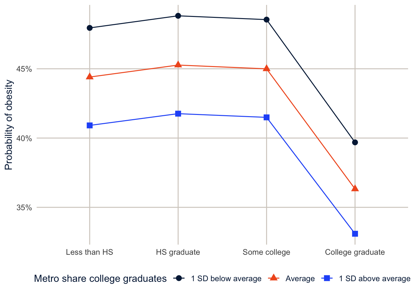

Figure 13.1: Predicted probability of obesity by education and metro share of college graduates, for a typical metro. NH White women aged 50.

expand_grid() builds every combination of education and three values of the metro education score (one standard deviation below average, average, one above), holding everything else fixed, as in week 11.

Part 2: Growth curve models

Time as a level-1 variable

In week 10, we treated the rounds of the ECLS-K as a nuisance and focused on the effect of poverty. A growth curve model makes change itself the outcome. It’s the same data structure as week 10, seen through week 12’s lens: repeated measurements are level 1 and children are level 2, and each child gets their own trajectory: an intercept (where they start) and a slope (how fast they grow), both random (Singer and Willett 2003). With time \(t\) for child \(i\):

\[y_{ti} = \pi_{0i} + \pi_{1i}t + \pi_{2i}t^2 + e_{ti}\] \[\pi_{0i} = \beta_{00} + \beta_{01}z_i + r_{0i}, \qquad \pi_{1i} = \beta_{10} + \beta_{11}z_i + r_{1i}\]

The second line is where it gets interesting: the starting point and the growth rate can depend on child characteristics \(z_i\). That’s a cross-level interaction between time and the child’s characteristics, and it’s exactly the random slope model from last week, with time as the slope.

Math growth from kindergarten to fifth grade

This time I’ll use all nine rounds of math scores, and SES measured at the start of kindergarten.

neg_to_na <- function(x) if_else(x < 0, NA_real_, as.numeric(x))

growth <- readRDS(here("data", "eclsk2011_k5.rds")) |>
  filter(w9c29p_9a0 > 0) |>
  select(childid, x_chsex_r, x_raceth_r, x12sesl,
         matches("^x[0-9]mscalk5$"), x1kage_r, x2kage_r, matches("^x[3-9]age$")) |>
  rename(x1age = x1kage_r, x2age = x2kage_r) |>
  pivot_longer(c(matches("mscalk5$"), matches("^x[0-9]age$")),
               names_to = c("round", ".value"),
               names_pattern = "x([0-9])(mscalk5|age)") |>
  mutate(round = as.integer(round),
         math = neg_to_na(mscalk5),
         age = neg_to_na(age) / 12,
         t = age - 5.5,                       # years since age 5.5
         female = as.numeric(x_chsex_r == 2),
         ses = neg_to_na(x12sesl),
         race = factor(case_when(x_raceth_r == 1 ~ "White", x_raceth_r == 2 ~ "Black",
                                 x_raceth_r %in% 3:4 ~ "Hispanic", x_raceth_r == 5 ~ "Asian",
                                 x_raceth_r > 5 ~ "Other"),
                       levels = c("White", "Black", "Hispanic", "Asian", "Other"))) |>
  filter(!is.na(math), !is.na(age), !is.na(race), !is.na(ses))

growth |> summarise(children = n_distinct(childid), observations = n())

#> # A tibble: 1 × 2
#>   children observations
#>      <int>        <int>
#> 1     4140        31333

NoteCode explanation: names_pattern

Here the round number comes before the variable name (x4mscalk5, x4age), so splitting at an underscore won’t work. names_pattern = "x([0-9])(mscalk5|age)" is a regular expression with two groups in parentheses: the first captures the digit, and the second captures either mscalk5 or age. Those two pieces go to names_to = c("round", ".value") in order, so the digit becomes the round, and the variable name becomes the column the value goes in. I renamed the two kindergarten age variables first, because their names (x1kage_r) don’t fit the pattern.

Children were tested at different ages within each round, so I use age, not round, as the time variable, centered at 5.5 years, which is about the average age at the fall kindergarten test. Where time starts, the time origin, decides what the intercept means: with \(t = 0\) at age 5.5, the intercept is the expected score at age 5.5, near the start of kindergarten, and the intercept variance describes how much children differ at that age. If I’d left age uncentered, the intercept would be the expected score at age 0, which means nothing for a math test. Always say where time starts.

gc0 <- lmer(math ~ t + I(t^2) + (1 + t | childid), data = growth,
            control = lmerControl(optimizer = "bobyqa"))
gc1 <- lmer(math ~ (t + I(t^2)) * (race + ses) + female + (1 + t | childid), data = growth,
            control = lmerControl(optimizer = "bobyqa"))

summary(gc0)$coefficients

#>              Estimate Std. Error   t value
#> (Intercept) 39.161969 0.23074318  169.7210
#> t           27.805312 0.07894456  352.2131
#> I(t^2)      -2.149508 0.01235665 -173.9556

VarCorr(gc0)

#>  Groups   Name        Std.Dev. Corr   
#>  childid  (Intercept) 13.7588         
#>           t            1.9402  -0.289 
#>  Residual              6.2827

(1 + t | childid) gives each child a random intercept and a random slope on time, as in week 12. In gc1, (t + I(t^2)) * (race + ses) lets both the linear and quadratic time terms differ by race and SES, which is how the trajectories are allowed to differ between groups.

The average child scores 39.2 at age 5.5 and gains 27.8 points a year at that age. The negative quadratic term says the gains slow down: by age 10, the annual gain is about 8.5 points. Children vary a lot in where they start (a standard deviation of 13.8 points) and somewhat in how fast they grow (1.9 points a year). The correlation between intercepts and slopes is -0.29: children who start higher grow a little more slowly, which is partly a ceiling effect on the test.

nd_g <- expand_grid(t = seq(-0.5, 5.5, by = 0.25), race = levels(growth$race),
                    ses = 0, female = 0.5)

nd_g |>
  mutate(math = predict(gc1, newdata = nd_g, re.form = NA),
         age = t + 5.5,
         race = factor(race, levels = levels(growth$race))) |>
  ggplot(aes(x = age, y = math, colour = race, linetype = race)) +
  geom_line(linewidth = 1.1) +
  scale_colour_utsa() +
  labs(x = "Age", y = "Predicted math scale score", colour = NULL, linetype = NULL)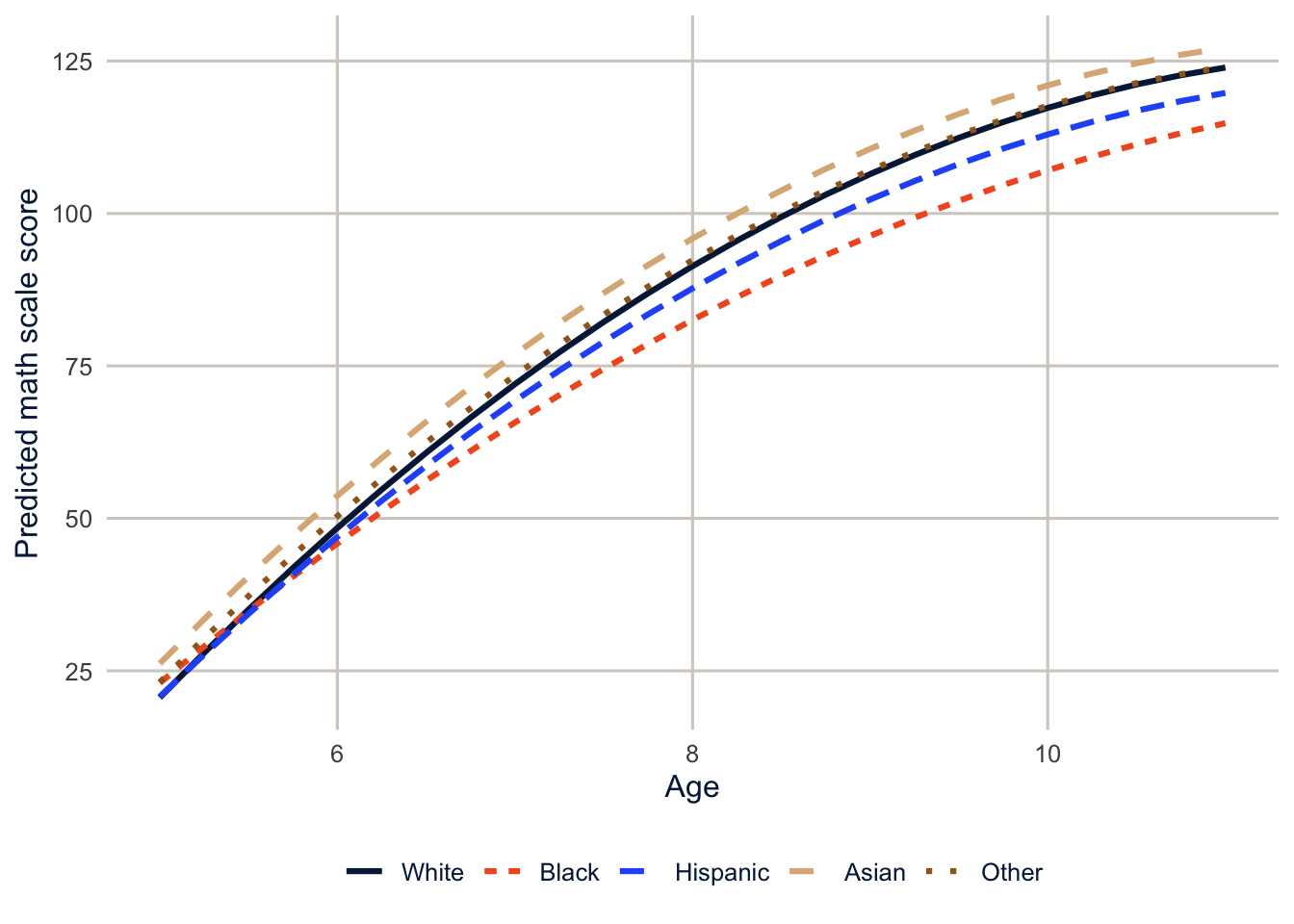

Figure 13.2: Predicted math growth by race and ethnicity, for children of average SES, from age 5 to 11.

Among children of the same SES, Black and White children start kindergarten close together, a gap of 0.2 points at age 5.5, but by age 10.5 the gap is 9.8 points, because Black children’s scores grow more slowly. That’s the kind of finding a growth curve model is built for: the gap isn’t something children bring to school, it opens up during the school years. The coefficients on t:ses say the same about SES: higher-SES children both start higher and grow faster.

Part 3: Age, period and cohort (extension)

The identification problem

Demographers have long wanted to separate three kinds of time. Age effects are changes that come with getting older. Period effects affect everyone alive at a given time, like a recession or a new medication. Cohort effects are shared by people born at the same time, who grew up in the same conditions and carry them through their lives. The problem is that the three are linked by an identity:

\[\text{cohort} = \text{period} - \text{age}\]

Take one person: interviewed in the 2010 survey (period) at age 40, she was born in 1970 (cohort). Interview her again in 2014 and she’s 44; her cohort is still 1970. Once you know her age and the survey year, her birth cohort is fixed. That’s the problem in a nutshell: if you know any two, you know the third, so a model with linear terms for all three can’t be estimated: there are infinitely many combinations of age, period and cohort slopes that fit the data equally well. Here it is in the NHIS, with BMI for adults from 2000 to 2014 (the subset is built by R/make_nhis_subset.R).

nhis <- readRDS(here("data", "nhis_2000_2014_adults.rds")) |>
  filter(BMICALC > 0, BMICALC < 990, BIRTHYR < 9997, AGE < 85) |>
  mutate(bmi = BMICALC, year = YEAR, age = AGE, cohort = BIRTHYR,
         cohort5 = floor(cohort / 5) * 5,
         female = as.numeric(SEX == 2))

lm(bmi ~ age + year + I(year - age), data = nhis) |> coef()

#>   (Intercept)           age          year I(year - age) 
#> -129.79202464    0.02922221    0.07751790            NA

floor(cohort / 5) * 5 rounds each birth year down to the start of its five-year group (1962 becomes 1960). The filter() drops the NHIS codes for missing values (BMI 0 or 990 and over, birth year 9997 and over).

R drops one of the three, because cohort is a linear combination of the other two. (I used year - age for cohort here. The reported birth year differs from it by up to a year, depending on whether the person had had their birthday yet at the interview, and that tiny difference is enough to let lm() estimate all three coefficients. The estimates would be meaningless, driven entirely by the timing of birthdays, which is a good illustration of how fragile “solutions” to this problem can be.) Any solution to the APC problem has to add information from outside the data, in the form of an assumption, a constraint, or a model that treats the three differently.

The hierarchical APC model

Yang and Land (2006; see also Yang and Land 2013) proposed a multilevel solution, the hierarchical APC (HAPC) model. Treat age as a fixed effect at the individual level, and treat period and cohort as crossed random effects: each person belongs to one survey year and one birth cohort, and the years and cohorts are two separate sets of groups.

\[y_{ijk} = \beta_0 + f(\text{age}_i) + \sum_c \beta_c x_{ic} + u_j + v_k + e_{ijk}, \qquad u_j \sim N(0, \sigma^2_u),\; v_k \sim N(0, \sigma^2_v)\]

where \(u_j\) is the effect of period \(j\) and \(v_k\) the effect of cohort \(k\). Using different functional forms (fixed versus random) and grouping cohorts into 5-year groups breaks the exact linear dependence, so the model can be estimated.

hapc <- lmer(bmi ~ ns(age, df = 4) + female + (1 | year) + (1 | cohort5), data = nhis, REML = FALSE)
VarCorr(hapc)

#>  Groups   Name        Std.Dev.
#>  cohort5  (Intercept) 0.11086 
#>  year     (Intercept) 0.34387 
#>  Residual             5.12842

I fit these models by maximum likelihood (REML = FALSE), not the default REML, because below I compare the log-likelihoods of models with different fixed effects, and REML likelihoods can’t be compared that way.

NoteCode explanation: crossed random effects

(1 | year) + (1 | cohort5) gives every survey year and every 5-year birth cohort its own random intercept. These are crossed, not nested: people born in 1960 appear in every survey year, and every survey year includes people from many cohorts. lmer() handles crossed random effects without any special syntax, as long as the two grouping variables are separate.

Why the HAPC model doesn’t solve the problem

The HAPC model was widely used, and then heavily criticized. Bell and Jones (2014), Luo (2013) and Fosse and Winship (2019), among others, show that treating period and cohort as random doesn’t identify anything; it just hides the constraint. Random effects are shrunk toward zero, so a linear trend in period or cohort, which is exactly the thing that can’t be identified, gets pushed somewhere by the model’s assumptions, not by the data. Look at the predicted period effects from the model above.

as.data.frame(ranef(hapc, condVar = TRUE)) |>
  filter(grpvar == "year") |>
  mutate(year = as.numeric(as.character(grp))) |>
  ggplot(aes(x = year, y = condval)) +
  geom_hline(yintercept = 0, colour = utsa_cols("smoke")) +
  geom_pointrange(aes(ymin = condval - 1.96 * condsd, ymax = condval + 1.96 * condsd),
                  colour = utsa_cols("midnight")) +
  labs(x = "Survey year", y = "Period effect on BMI")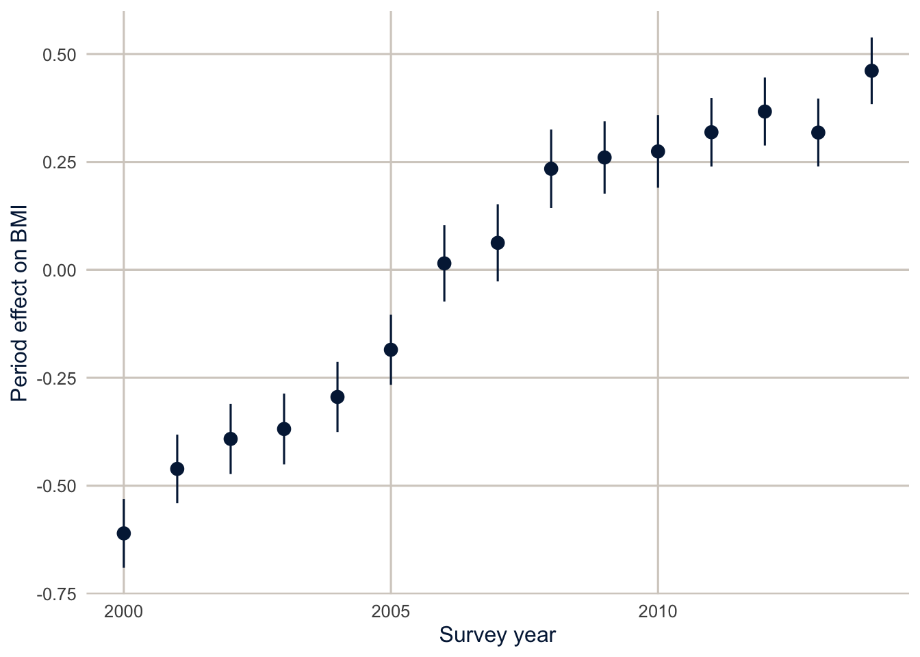

Figure 13.3: Predicted period effects from the HAPC model, with 95% intervals.

The “random” period effects are a nearly straight line from -0.61 in 2000 to 0.46 in 2014. That violates the assumption that they’re independent draws from a normal distribution, and it means the model has put the upward trend in BMI in the period effects. Nothing in the data says it belongs there rather than in the cohort effects. To see this, add a linear cohort trend as a fixed effect, which is perfectly legal, and compare the fit and the age curve.

hapc_cohort <- lmer(bmi ~ ns(age, df = 4) + female + I((cohort - 1950) / 10) +
                      (1 | year) + (1 | cohort5), data = nhis, REML = FALSE)

c(logLik_hapc = as.numeric(logLik(hapc)), logLik_with_cohort_trend = as.numeric(logLik(hapc_cohort)))

#>              logLik_hapc logLik_with_cohort_trend 
#>                 -1162864                 -1162862

logLik() returns a model’s log-likelihood; higher is a better fit. I((cohort - 1950) / 10) adds a linear cohort trend, in decades since 1950, as a fixed effect.

nd_a <- tibble(age = 20:80, female = 0.5, cohort = 1950)

nd_a |>
  mutate(`HAPC` = predict(hapc, newdata = nd_a, re.form = NA),
         `HAPC with a linear cohort trend` = predict(hapc_cohort, newdata = nd_a, re.form = NA)) |>
  pivot_longer(-c(age, female, cohort), names_to = "model", values_to = "bmi") |>
  ggplot(aes(x = age, y = bmi, colour = model, linetype = model)) +
  geom_line(linewidth = 1.1) +
  scale_colour_utsa(palette = "primary") +
  labs(x = "Age", y = "Predicted BMI", colour = NULL, linetype = NULL)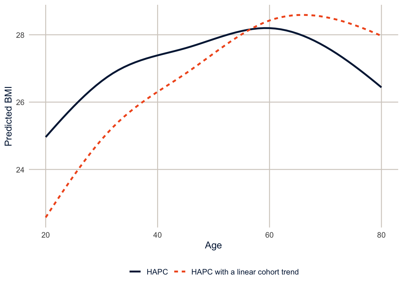

Figure 13.4: Predicted age curves for BMI from two HAPC specifications that fit the data almost equally well.

The two models fit the data almost identically (their log-likelihoods differ by 2.1 points out of hundreds of thousands), but they tell different stories about aging. The first says BMI rises 3.2 points from age 20 to 60, and the second says 5.8. Shifting a linear trend into the cohort term made the age curve steeper, and the period effects flatter. Neither is wrong, and the data can’t choose between them. That’s the identification problem, still there, hidden inside the random effects. Any fitted age, period or cohort curve depends on a constraint or assumption, whether it’s stated or hidden in the model’s structure, and should be labeled that way.

What to do instead

There’s no technical fix, so the advice from the recent literature (Fosse and Winship 2019; Luo and Hodges 2022) is about being explicit.

1. Say which assumption you’re making, and why. If you have a substantive reason to believe there’s no linear period trend (or that the cohort effect is zero beyond some point), state it, and use it as your constraint. That’s the only way to identify the linear components.
2. Interpret the nonlinear parts. Deviations from linear trends (accelerations, bumps, a cohort that’s unusually high or low compared with its neighbors) are identified, regardless of the constraint. A change in the slope of the period effects after a policy change is real information.
3. Look for mechanisms. Replace “period” or “cohort” with something measured that you think explains it: the obesity rate in the person’s state when they were 18, or food prices in the survey year. Then the question isn’t an APC problem anymore.
4. Do sensitivity analyses. Show how much the conclusions change under different reasonable constraints, as the figure above does.

Summary

Generalized linear mixed models extend multilevel models to binary, count and other outcomes, with the latent-scale ICC and the median odds ratio to describe how much places matter. They’re slower and more fragile than linear mixed models, so rescale predictors and try other optimizers when they don’t converge. Growth curve models are random slope models with time at level 1, and cross-level interactions with time show how trajectories differ between groups. Hierarchical APC models are multilevel models with crossed random effects for period and cohort, but they don’t solve the age-period-cohort identification problem; they hide it, and different specifications that fit equally well can give different answers. The only honest approaches are explicit assumptions, a focus on the nonlinear components, measured mechanisms, and sensitivity analyses.

Homework 13

Due: April 22, before class.

Which version to do. If you’re in DEM 7283, do the version with your own survey data. If you’re in DEM 5283, do either version, and say at the top of your homework which one you did. If your survey can’t support this week’s method, do the version with my data and say so.

Purpose. Extend multilevel models to a binary outcome and to growth over time, and report what they show without overstating it.

A satisfactory answer reports predicted probabilities and says whether they’re for a typical metro or averaged over metros; states where time starts in any growth model; and, for exercise 4, explains competing interpretations instead of picking one by fit statistics.

With your own survey data

Use the full survey design for every estimate unless a step says otherwise, and report each estimate with a standard error or confidence interval.

1. Using the grouping variable from Homework 12 (or the chapter’s data), fit a generalized linear mixed model for a binary outcome with glmer().
   1. Start with a random intercept only model and report the ICC on the latent scale.
   2. Add individual-level and group-level predictors, and present the results as odds ratios with confidence intervals.
2. Report predicted probabilities for some interesting cases, and explain the difference between predictions for a typical group (random effect set to zero) and predictions averaged over groups.
3. Compare the GLMM’s fixed effects with a svyglm() logit for the same outcome and predictors. Why are the GLMM’s coefficients typically larger in magnitude?
4. Growth curves. Using repeated measurements (from your data, or the ECLS-K data from the chapter), fit a growth curve model with time as a level-1 variable.
   1. Fit random intercepts, then random intercepts and slopes for time.
   2. Does the shape of growth need to be nonlinear? Try a quadratic or spline term for time.
   3. Add a time-constant predictor and its interaction with time, and interpret it.
   4. Plot the predicted trajectories for two groups.

With my data

What is provided. The BRFSS data with metro context and the GLMM glmm1, the ECLS-K growth data growth and models gc0 and gc1, and (for the extension) the NHIS data and HAPC models from this chapter.

1. Add a cross-level interaction between race and ethnicity and the metro poverty rate (race_eth * z_pct_poverty) to the obesity GLMM. Are the racial and ethnic differences in obesity larger in poorer metros? Show the answer as predicted probabilities, not odds ratios.

# YOUR CODE HERE

2. Fit the growth curve model for reading scores (x1rscalk5 to x9rscalk5). Does the Black-White gap in reading grow the same way as the gap in math?

# YOUR CODE HERE

One solution for exercise 2

growth_read <- readRDS(here("data", "eclsk2011_k5.rds")) |>
  filter(w9c29p_9a0 > 0) |>
  select(childid, x_chsex_r, x_raceth_r, x12sesl,
         matches("^x[0-9]rscalk5$"), x1kage_r, x2kage_r, matches("^x[3-9]age$")) |>
  rename(x1age = x1kage_r, x2age = x2kage_r) |>
  pivot_longer(c(matches("rscalk5$"), matches("^x[0-9]age$")),
               names_to = c("round", ".value"), names_pattern = "x([0-9])(rscalk5|age)") |>
  mutate(read = neg_to_na(rscalk5), t = neg_to_na(age) / 12 - 5.5,
         female = as.numeric(x_chsex_r == 2), ses = neg_to_na(x12sesl),
         race = factor(case_when(x_raceth_r == 1 ~ "White", x_raceth_r == 2 ~ "Black",
                                 x_raceth_r %in% 3:4 ~ "Hispanic", x_raceth_r == 5 ~ "Asian",
                                 x_raceth_r > 5 ~ "Other"),
                       levels = c("White", "Black", "Hispanic", "Asian", "Other"))) |>
  filter(!is.na(read), !is.na(t), !is.na(race), !is.na(ses))

gc_read <- lmer(read ~ (t + I(t^2)) * (race + ses) + female + (1 + t | childid),
                data = growth_read, control = lmerControl(optimizer = "bobyqa"))
summary(gc_read)$coefficients[c("raceBlack", "t:raceBlack", "I(t^2):raceBlack"), ]

3. In the growth curve model, replace the quadratic in time with a natural spline, ns(t, df = 3), interacted with race (keep the random slope on linear t). Do the predicted trajectories change much?

# YOUR CODE HERE

4. (Extension.) First, explain the APC identity in your own words, using an example person. Then refit the HAPC model with a linear period trend as a fixed effect instead of a cohort trend, and compare its age curve and cohort effects with the two models above. Identify the assumption that differs between the specifications. In a paragraph, explain to a skeptical reader why the different fitted age or cohort patterns don’t show that one specification recovered the true effects, and why choosing the one with the best fit statistics wouldn’t settle it.

# YOUR CODE HERE

Additional resources

• Ben Bolker’s GLMM FAQ is the first place to look when glmer() warns you about convergence or singular fits.
• Austin and Merlo (2017) is a tutorial on intermediate and advanced multilevel logistic regression, including the ICC and the median odds ratio from this chapter.
• Fosse and Winship (2019), in the Annual Review of Sociology, reviews the age-period-cohort identification problem and why no statistical model can solve it.
• The brms documentation has vignettes on Bayesian multilevel models, for when glmer() won’t converge or you have few groups.

Austin, Peter C., and Juan Merlo. 2017. “Intermediate and Advanced Topics in Multilevel Logistic Regression Analysis.” Statistics in Medicine 36 (20): 3257–77.

Bell, Andrew, and Kelvyn Jones. 2014. “Another ‘Futile Quest’? A Simulation Study of Yang and Land’s Hierarchical Age-Period-Cohort Model.” Demographic Research 30 (11): 333–60.

Fosse, Ethan, and Christopher Winship. 2019. “Analyzing Age-Period-Cohort Data: A Review and Critique.” Annual Review of Sociology 45: 467–92.

Luo, Liying. 2013. “Assessing Validity and Application Scope of the Intrinsic Estimator Approach to the Age-Period-Cohort Problem.” Demography 50 (6): 1945–67.

Luo, Liying, and James S. Hodges. 2022. “The Age-Period-Cohort-Interaction Model for Describing and Investigating Inter-Cohort Deviations and Intra-Cohort Life-Course Dynamics.” Sociological Methods & Research 51 (3): 1164–210.

Merlo, Juan, Basile Chaix, Henrik Ohlsson, et al. 2006. “A Brief Conceptual Tutorial of Multilevel Analysis in Social Epidemiology: Using Measures of Clustering in Multilevel Logistic Regression to Investigate Contextual Phenomena.” Journal of Epidemiology and Community Health 60 (4): 290–97.

Singer, Judith D., and John B. Willett. 2003. Applied Longitudinal Data Analysis: Modeling Change and Event Occurrence. Oxford University Press.

Yang, Yang, and Kenneth C. Land. 2006. “A Mixed Models Approach to the Age-Period-Cohort Analysis of Repeated Cross-Section Surveys, with an Application to Data on Trends in Verbal Test Scores.” Sociological Methodology 36: 75–97.

Yang, Yang, and Kenneth C. Land. 2013. Age-Period-Cohort Analysis: New Models, Methods, and Empirical Applications. CRC Press.