library(tidyverse)
library(here)
library(survey)
library(splines)
library(mgcv)
library(ipumsr)
library(sparkscolors)  # pak::pak("coreysparks/sparkscolors"), UTSA colors

source(here("R", "get_mmsa.R"))
source(here("R", "recode_mmsa.R"))Week 11: Splines and Generalized Additive Models
Introduction
Demographers spend a lot of time on age, and almost nothing important is a straight line in age. Mortality falls through childhood and rises exponentially in adulthood, fertility rises and falls, earnings grow fast early in a career and level off, and self-rated health declines in a pattern that’s anything but linear. So far we’ve handled curves by cutting age into groups, which throws away information and makes the curve a staircase, or by adding \(x^2\), which forces the curve to be a parabola, symmetric around its peak.
Splines are a better way. A spline is a set of simple functions (lines or cubic polynomials) joined together at points called knots. The knots are just the places where one piece ends and the next begins, and the spline is built with smoothness constraints that force the pieces to meet without a jump or a sharp corner, so together they form one coherent curve. That lets the curve bend where the data bend and stay smooth everywhere. This week covers regression splines, which you can drop into any model we’ve used, including survey-weighted ones, and generalized additive models (GAMs), which choose how wiggly each curve should be from the data.
The useful result of a spline model is almost never its coefficients. It’s the predicted curve and its uncertainty, so that’s what we’ll look at throughout.
NoteThis week at a glance
The question. How does the probability of fair or poor health change across ages, and does the pattern differ by education?
By the end of this week you should be able to
- explain what knots, a spline basis and a smoothing penalty are, and why the curve, not the coefficients, is what you interpret;
- compare a straight line, a quadratic and a spline for the same outcome, and choose the flexibility with an eye to both missing a pattern and following noise;
- describe a nonlinear age pattern from cross-sectional data without claiming it shows how individuals change as they age.
Before you begin. You need survey-weighted logit models and predictions from week 3, the design-based model comparison with anova() from week 4, and the IPUMS wage data from week 7.
Required and optional. Everything is required. The equations for the spline pieces are there to show the idea; you won’t need to write them.
Setup
The splines package comes with R and makes spline terms for any regression formula. mgcv fits GAMs (Wood 2017).
Splines
Piecewise linear splines
In the simplest case, the relationship between \(x\) and \(y\) changes at one point. Here are some simulated data where \(y\) rises with \(x\) until \(x = 70\) and then levels off.
set.seed(7283)
sim1 <- tibble(x = 1:100,
               y = c(rnorm(70, 1 + 0.5 * (1:70), 1), rnorm(30, 35, 1)))

fit_line <- lm(y ~ x, data = sim1)
rnorm(70, 1 + 0.5 * (1:70), 1) draws 70 Normal values whose means rise by 0.5 at each step, and rnorm(30, 35, 1) draws 30 more around a flat 35, so the true line rises and then levels off at 70. c() joins them.
A straight line through these data misses the change completely. Instead, we can let the line bend at a knot. Mathematically, a spline with knots \(x_1, x_2, \ldots, x_k\) is a set of functions, one for each interval between knots:
\[f(x) = \begin{cases} F_1(x) & \text{for } x \in [x_1, x_2] \\ F_2(x) & \text{for } x \in [x_2, x_3] \\ \quad\vdots \\ F_{k}(x) & \text{for } x \in [x_{k-1}, x_k] \end{cases}\]
joined so that they meet at the knots. For a linear spline with one knot at \(c\), that’s just one extra term in the regression, \((x - c)_+\), which is 0 below the knot and \(x - c\) above it:
\[y = \beta_0 + \beta_1 x + \beta_2 (x - c)_+ + \varepsilon\]
Below the knot the slope is \(\beta_1\), and above it the slope is \(\beta_1 + \beta_2\).
fit_knot <- lm(y ~ x + pmax(x - 70, 0), data = sim1)

sim1 |>
  mutate(`Straight line` = fitted(fit_line), `Spline, knot at 70` = fitted(fit_knot)) |>
  pivot_longer(c(`Straight line`, `Spline, knot at 70`), names_to = "model", values_to = "fitted") |>
  ggplot(aes(x = x)) +
  geom_point(aes(y = y), colour = utsa_cols("smoke")) +
  geom_line(aes(y = fitted, colour = model, linetype = model), linewidth = 1.2) +
  scale_colour_utsa(palette = "primary") +
  labs(colour = NULL, linetype = NULL)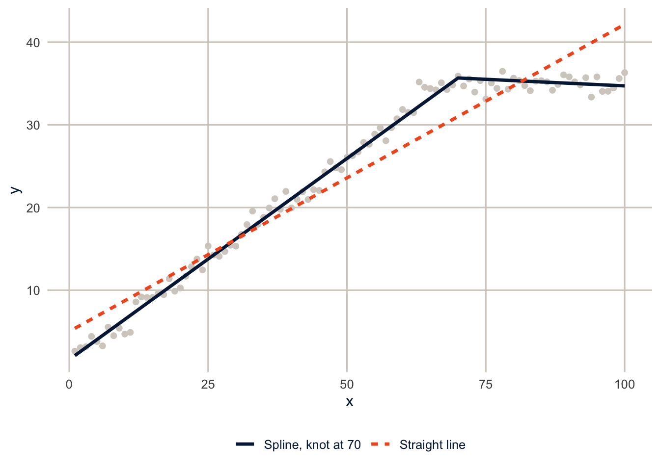
NoteCode explanation:
pmax(x - 70, 0)
pmax() is the “parallel maximum”: it compares two vectors element by element and keeps the larger value. pmax(x - 70, 0) is 0 when x is below 70 (because x - 70 is negative) and x - 70 above it, which is exactly \((x - c)_+\). You can put a function like this directly in a model formula.
The slope below the knot is 0.49 (the true value is 0.5), and above it is -0.03 (the true value is 0). The spline found the change because I told it where to look. Usually we don’t know where the knots should go, and the curve isn’t made of straight pieces.
Cubic splines and more knots
Most real curves are smooth, and pieces of straight lines have corners. Cubic splines use a cubic polynomial between each pair of knots, joined so that the curve and its first two derivatives are continuous at the knots, which makes the joins invisible. Here is a noisier curve, a sine wave, with cubic splines that use more and more flexibility.
set.seed(7283)
sim2 <- tibble(t = seq(0, 2 * pi, length.out = 200),
               y = 3 * sin(2 * t) + rnorm(200, 0, 2))

sim2 |>
  mutate(`Straight line` = fitted(lm(y ~ t)),
         `3 df` = fitted(lm(y ~ bs(t, df = 3))),
         `6 df` = fitted(lm(y ~ bs(t, df = 6))),
         `20 df` = fitted(lm(y ~ bs(t, df = 20)))) |>
  pivot_longer(-c(t, y), names_to = "model", values_to = "fitted") |>
  mutate(model = fct_inorder(model)) |>
  ggplot(aes(x = t)) +
  geom_point(aes(y = y), colour = utsa_cols("smoke")) +
  geom_line(aes(y = fitted, colour = model, linetype = model), linewidth = 1.1) +
  scale_colour_utsa() +
  labs(colour = NULL, linetype = NULL)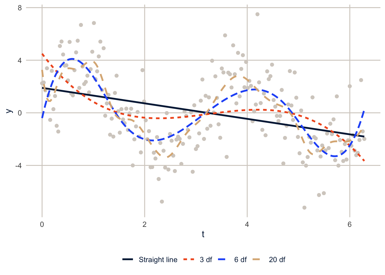
With 3 degrees of freedom (a plain cubic), the curve can’t follow the data. With 6 it captures the wave. With 20 it starts chasing the noise. That’s the basic tradeoff with splines: too little flexibility misses a real pattern, and too much follows the noise in this particular sample, which wouldn’t be there in another sample. Every method below is a way of deciding how much flexibility to allow, and none of them removes the uncertainty in that choice. Two reasonable choices can give somewhat different curves, which is worth checking (exercise 1 does).
seq(0, 2 * pi, length.out = 200) makes 200 evenly spaced values from 0 to \(2\pi\), and fitted() returns each model’s fitted values.
B-splines and natural splines
In R, you add a spline to a model formula with bs() (a B-spline) or ns() (a natural spline). Both turn one variable into several columns, called the basis, and the model estimates a coefficient for each column. The fitted curve is the sum of the columns times their coefficients.
age_grid <- 18:80
basis <- ns(age_grid, df = 4)

as_tibble(unclass(basis)[, 1:4]) |>
  set_names(paste("Basis", 1:4)) |>
  mutate(age = age_grid) |>
  pivot_longer(-age, names_to = "column", values_to = "value") |>
  ggplot(aes(x = age, y = value, colour = column, linetype = column)) +
  geom_line(linewidth = 1.1) +
  scale_colour_utsa() +
  labs(x = "Age", y = "Basis value", colour = NULL, linetype = NULL)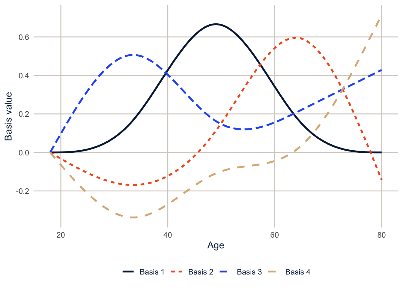
NoteCode explanation:
bs() and ns()
bs(x, df = 6)makes a cubic B-spline basis with 6 columns. Withdfand noknots, R puts the knots at evenly spaced quantiles ofx, so there are more knots where there are more data. You can also give the knots yourself, as inbs(x, knots = c(30, 50, 65)).ns(x, df = 4)makes a natural cubic spline basis. A natural spline is constrained to be a straight line beyond the outermost knots. Cubic polynomials tend to swing wildly at the edges of the data, where there are fewer observations, and the natural spline stops that. For age, I almost always usens().- The individual coefficients on these columns don’t mean anything you’d want to interpret. Interpret the curve, by predicting from the model over a range of values, as we’ll do below.
- In the figure code,
unclass(basis)strips the spline’s special class so it can be treated as an ordinary matrix and turned into a data frame.
A natural spline also tells you something about extrapolation: what the curve does beyond the data. It just continues in a straight line, which is a guess, not a finding. Any curve, spline or not, is only supported by data where there are data. The BRFSS top-codes age at 80, so nothing here says anything about health at 90.
How many degrees of freedom? Harrell (2015) suggests 3 to 5 knots for most problems, which is 4 to 6 degrees of freedom, and says that where the knots go matters much less than how many there are. You can also compare models with AIC, or let the data decide, which is what a GAM does.
Self-rated health and age in the BRFSS
Here is the probability of reporting fair or poor health by age, in a survey-weighted logit model with a straight line in age and with a natural spline. The BRFSS gives age in single years, top-coded at 80.
brfss <- get_mmsa() |>
  recode_mmsa() |>
  mutate(age = age80)

des <- svydesign(ids = ~1, strata = ~ststr, weights = ~mmsawt, data = brfss)

fit_linear <- svyglm(badhealth ~ age + female + educ + race_eth,
                     design = des, family = quasibinomial)
fit_quadratic <- svyglm(badhealth ~ age + I(age^2) + female + educ + race_eth,
                        design = des, family = quasibinomial)
fit_spline <- svyglm(badhealth ~ ns(age, df = 4) + female + educ + race_eth,
                     design = des, family = quasibinomial)

anova(fit_linear, fit_spline)
#> Working (Rao-Scott+F) LRT for ns(age, df = 4) - age
#> in svyglm(formula = badhealth ~ ns(age, df = 4) + female + educ +
#> race_eth, design = des, family = quasibinomial)
#> Working 2logLR = 30.9821 p= 1.1289e-06
#> (scale factors: 1.1 1 0.88 ); denominator df= 223011The linear model and the spline are nested (a straight line is a special case of the spline), so the design-based likelihood ratio test from week 4 compares them, and it strongly prefers the spline. To see what the three shapes do, predict over the age range. These curves hold the other variables at fixed values: a non-Hispanic White woman with a high school education. They describe that kind of person at each age, not the average over the whole population; for a population average at each age, you’d use avg_predictions() from week 3 instead.
newdat <- tibble(age = 18:80, female = 1, educ = "HS graduate", race_eth = "NH White")

predict_curve <- function(fit, label) {
  p <- predict(fit, newdata = newdat, type = "link", se.fit = TRUE)
  newdat |>
    mutate(model = label,
           fit = plogis(coef(p)),
           lower = plogis(coef(p) - 1.96 * SE(p)),
           upper = plogis(coef(p) + 1.96 * SE(p)))
}

curves <- bind_rows(predict_curve(fit_linear, "Linear in age"),
                    predict_curve(fit_quadratic, "Quadratic in age"),
                    predict_curve(fit_spline, "Natural spline, 4 df")) |>
  mutate(model = fct_inorder(model))

ggplot(curves, aes(x = age, y = fit, colour = model, fill = model, linetype = model)) +
  geom_ribbon(aes(ymin = lower, ymax = upper), alpha = 0.2, colour = NA) +
  geom_line(linewidth = 1.1) +
  scale_colour_utsa() +
  scale_fill_utsa() +
  scale_y_continuous(labels = scales::label_percent()) +
  labs(x = "Age", y = "Probability of fair or poor health",
       colour = NULL, fill = NULL, linetype = NULL)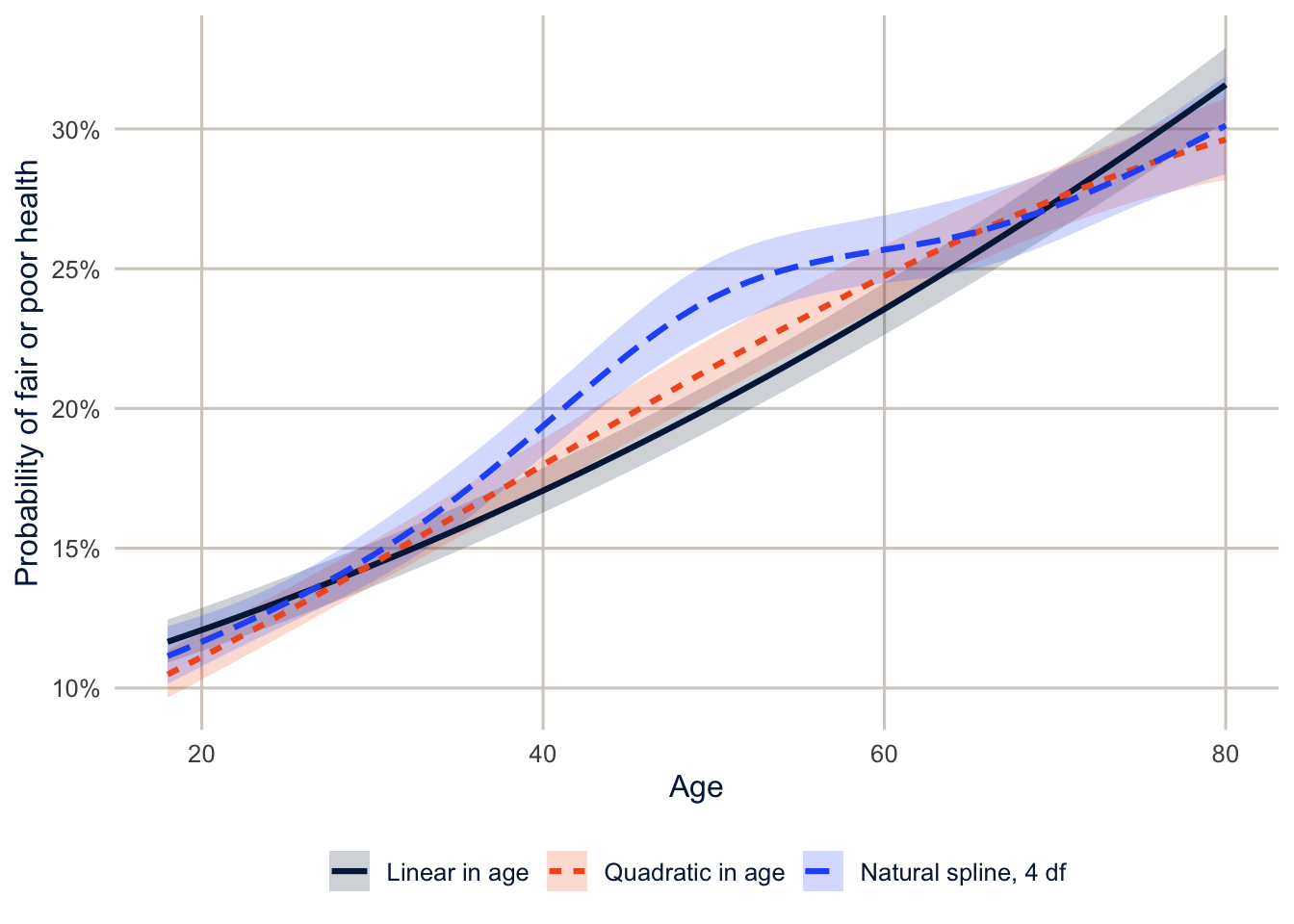
NoteCode explanation: predictions with confidence bands
predict()on asvyglmwithse.fit = TRUEreturns the predictions and their design-based standard errors.coef(p)andSE(p)pull them out.- I predict on the link (log-odds) scale, build the 95% interval there, and convert everything to probabilities with
plogis(). Building the interval on the probability scale could give limits below 0 or above 1. predict_curve()wraps those steps in a function so I can do the same thing to both models, andbind_rows()stacks the results for plotting.
The straight line says the probability rises steadily with age. The quadratic can bend, but only into a single symmetric arc (on the log-odds scale). The spline says something more interesting: among adults of different ages in 2024, fair or poor health is more common at each older age through the 30s, 40s and early 50s, then nearly flat from the mid-50s to the mid-60s before rising again. The straight line averages over all of that.
Be careful about why. These are different people of different ages, measured once, not the same people followed as they age. A cross-sectional age pattern mixes three things: what happens to people as they age; cohort differences between people born in different decades (today’s 60-year-olds grew up with different diets, jobs and health care than today’s 30-year-olds); and selection, since the people in the worst health have died or moved into nursing homes and aren’t answering phone surveys. The flat stretch could come from any of these, including people leaving the labor force around those ages. The curve describes the pattern; it can’t tell you how a person’s health changes as they age.
TipReading the result: a right and a wrong interpretation
Right: “In 2024, the predicted probability of fair or poor health is higher at each older age through the early 50s, then roughly flat between the mid-50s and mid-60s, among otherwise similar adults.”
Wrong: “People’s health stops declining in their late 50s and early 60s.” That’s a claim about individuals changing over time, and these data compare different people of different ages at one time. To see how individuals change, you need longitudinal data (week 10), and even then, separating age from cohort is the hard problem of week 13.
Does the age pattern differ by education?
A spline can interact with other variables like any other term. Here the age curve is allowed to differ by education.
fit_spline_educ <- svyglm(badhealth ~ ns(age, df = 4) * educ + female + race_eth,
                          design = des, family = quasibinomial)
anova(fit_spline, fit_spline_educ)
#> Working (Rao-Scott+F) LRT for ns(age, df = 4):educ
#> in svyglm(formula = badhealth ~ ns(age, df = 4) * educ + female +
#> race_eth, design = des, family = quasibinomial)
#> Working 2logLR = 81.96153 p= 6.2808e-10
#> (scale factors: 1.6 1.6 1.3 1.3 1 0.95 0.88 0.83 0.71 0.68 0.61 0.54 ); denominator df= 222999newdat_educ <- expand_grid(age = 18:80, educ = levels(brfss$educ),
female = 1, race_eth = "NH White")
newdat_educ |>
mutate(fit = as.numeric(predict(fit_spline_educ, newdata = newdat_educ, type = "response")),
educ = factor(educ, levels = levels(brfss$educ))) |>
ggplot(aes(x = age, y = fit, colour = educ, linetype = educ)) +
geom_line(linewidth = 1.1) +
scale_colour_utsa() +
scale_y_continuous(labels = scales::label_percent()) +
labs(x = "Age", y = "Probability of fair or poor health", colour = NULL, linetype = NULL)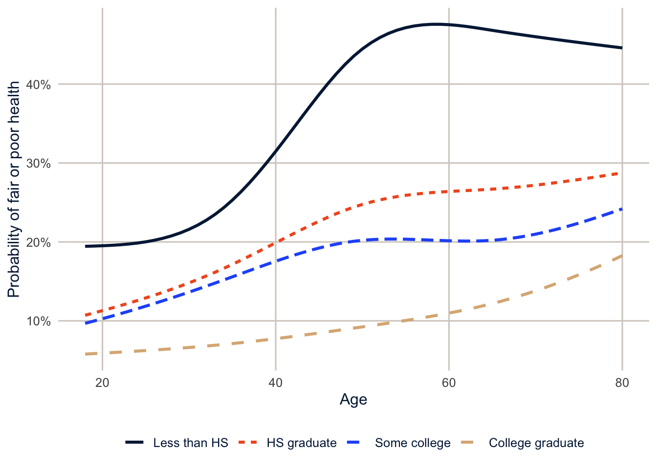
anova(fit_spline, fit_spline_educ) tests whether letting the curve differ by education improves the fit.
The education gap is already there among young adults, but it’s more than twice as large in midlife, and it’s largest in the late 50s and early 60s. That’s consistent with the pattern the cumulative advantage literature predicts, and you’d miss it with age groups or a single age slope. It’s also, for the same cross-sectional reasons as above, consistent with cohort differences in the meaning of education and with differential survival, so on its own it isn’t evidence that advantages accumulate within lives.
NoteCode explanation:
expand_grid()
expand_grid() makes every combination of the values you give it: here, every age from 18 to 80 for each of the four education levels, so 63 × 4 = 252 rows. Single values like female = 1 are repeated on every row. It’s the easiest way to build data for predictions.
Generalized additive models
Letting the data choose
With regression splines, you choose the degrees of freedom. A generalized additive model (Hastie and Tibshirani 1990; Wood 2017) estimates the curve and how wiggly it should be at the same time. The linear predictor is a sum of smooth functions and ordinary linear terms:
\[g(E(y)) = \beta_0 + f_1(x_1) + f_2(x_2) + \beta_3 x_3 + \cdots\]
Each \(f\) is a spline with many knots, but the model adds a penalty for wiggliness: the more the curve bends, the more it costs. Two separate things are going on, and it helps to keep them apart. The basis sets the maximum flexibility the curve could have (in mgcv, the argument k, which defaults to 10). The penalty decides how much of that flexibility the curve actually uses. A smoothing parameter sets the balance between fitting the data and staying smooth, and mgcv estimates it from the data. The result is summarized by the effective degrees of freedom (edf) of each smooth, a measure of how complex the fitted curve turned out to be. An edf near 1 means the curve is essentially a straight line, and larger values mean more bending. The edf doesn’t have to be a whole number, and it isn’t the number of knots: a basis with 9 knots might end up with an edf of 3 if the penalty keeps the curve simple.
Here’s the sine example again.
gam_sim <- gam(y ~ s(t), data = sim2)
summary(gam_sim)$s.table
#> edf Ref.df F p-value
#> s(t) 7.373247 8.355654 27.65105 0gam(y ~ s(t)) fits a GAM with a smooth function of t. summary(gam_sim)$s.table pulls the table of smooth terms out of the summary, with each smooth’s edf and a test of whether it’s flat.
The GAM used about 7.4 effective degrees of freedom, close to the 6 that looked right above, without being told.
A GAM for self-rated health
brfss_cc <- brfss |>
  filter(!is.na(badhealth), !is.na(educ), !is.na(race_eth)) |>
  mutate(w = mmsawt / mean(mmsawt))

gam_health <- bam(badhealth ~ s(age, by = educ) + educ + female + race_eth,
                  data = brfss_cc, weights = w, family = quasibinomial, discrete = TRUE)
summary(gam_health)$s.table
#> edf Ref.df F p-value
#> s(age):educLess than HS 7.138225 8.172397 166.90416 0
#> s(age):educHS graduate 7.969430 8.715583 177.83878 0
#> s(age):educSome college 7.676673 8.548731 98.52779 0
#> s(age):educCollege graduate 3.689054 4.559033 212.30387 0
NoteCode explanation:
bam() and s(age, by = educ)
gam()andbam()fit the same models.bam()(“big additive model”) is designed for large data sets, anddiscrete = TRUEspeeds it up further by rounding the covariates to a grid of values. With 224,220 respondents,bam()takes a couple of seconds andgam()takes much longer.s(age)is a smooth function of age.s(age, by = educ)fits a separate smooth for each education level. Because the smooths are centered at zero, you also need the main effect ofeducto let the levels differ in their averages.weights = wuses the survey weights, rescaled to average 1. The point estimates are weighted, but the standard errors are not design-based.mgcvdoesn’t know about strata or clusters. For design-based inference on a curve, usens()insvyglm()as above, and use the GAM to explore.
Like the earlier curves, the GAM predictions below hold sex and race and ethnicity fixed (a non-Hispanic White woman) and vary age and education.
The effective degrees of freedom for the college graduates’ curve are 3.7, compared with 7.1 to 8 for the others: their curve is smoother, without the same midlife acceleration.
newdat_educ |>
  mutate(fit = predict(gam_health, newdata = newdat_educ, type = "response"),
         educ = factor(educ, levels = levels(brfss$educ))) |>
  ggplot(aes(x = age, y = fit, colour = educ, linetype = educ)) +
  geom_line(linewidth = 1.1) +
  scale_colour_utsa() +
  scale_y_continuous(labels = scales::label_percent()) +
  labs(x = "Age", y = "Probability of fair or poor health", colour = NULL, linetype = NULL)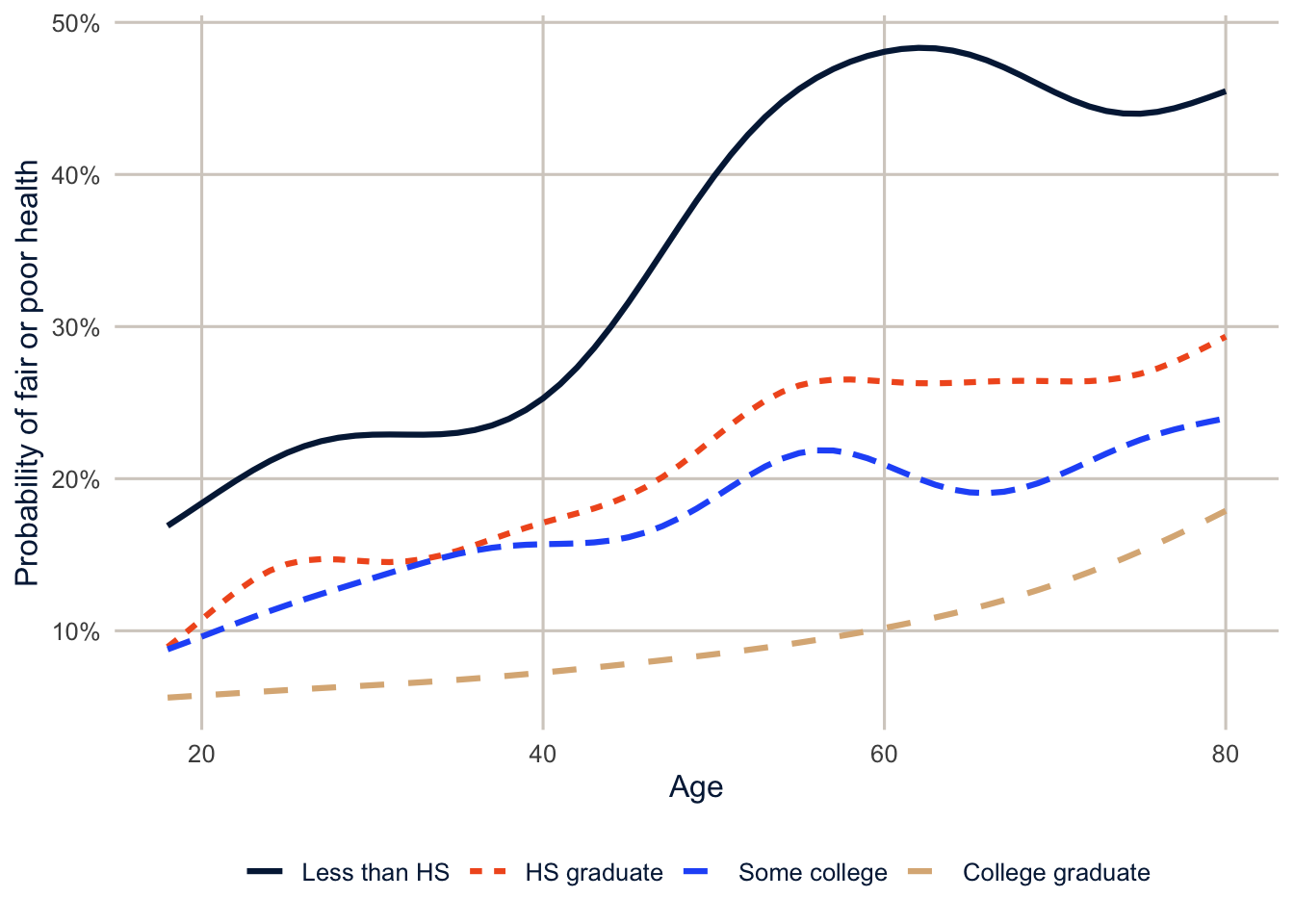
The GAM and the regression spline tell the same story, which is reassuring. The GAM wiggles a little more, because it’s free to.
The age-earnings profile
One of the oldest curves in social science is the relationship between age and earnings. Earnings rise quickly in the first years of a career, as people gain experience and change jobs, then flatten, and eventually fall as people cut back their hours or retire. The traditional model is a quadratic in age (or experience), which forces the curve to be a symmetric hill. Here’s the Texas ACS wage data from week 2, with a quadratic and a natural spline, separately for men and women.
ddi <- read_ipums_ddi(here("data", "usa_00014.xml"))
wages <- read_ipums_micro(ddi, data_file = here("data", "usa_00014_tx.dat.gz"),
                          verbose = FALSE) |>
  filter(EMPSTAT == 1, between(AGE, 18, 70), INCWAGE > 0, INCWAGE < 999998) |>
  mutate(lnwage = log(INCWAGE),
         sex = if_else(SEX == 2, "Women", "Men"))

fit_quad <- lm(lnwage ~ (AGE + I(AGE^2)) * sex, data = wages, weights = PERWT)
fit_ns <- lm(lnwage ~ ns(AGE, df = 6) * sex, data = wages, weights = PERWT)
AIC(fit_quad, fit_ns)
#> df AIC
#> fit_quad 7 372501.8
#> fit_ns 15 369323.3(AGE + I(AGE^2)) * sex interacts both the age and age-squared terms with sex, so men and women each get their own quadratic. In the hidden code that finds the peaks, which.max() gives the position of the largest prediction, and AGE[which.max(...)] the age at that position.
newdat_w <- expand_grid(AGE = 18:70, sex = c("Men", "Women"))

newdat_w |>
  mutate(Quadratic = exp(predict(fit_quad, newdata = newdat_w)),
         `Natural spline, 6 df` = exp(predict(fit_ns, newdata = newdat_w))) |>
  pivot_longer(c(Quadratic, `Natural spline, 6 df`), names_to = "model", values_to = "wage") |>
  ggplot(aes(x = AGE, y = wage, colour = model, linetype = model)) +
  geom_line(linewidth = 1.1) +
  facet_wrap(~sex) +
  scale_colour_utsa(palette = "primary") +
  scale_y_continuous(labels = scales::label_dollar()) +
  labs(x = "Age", y = "Predicted annual wage (geometric mean)", colour = NULL, linetype = NULL)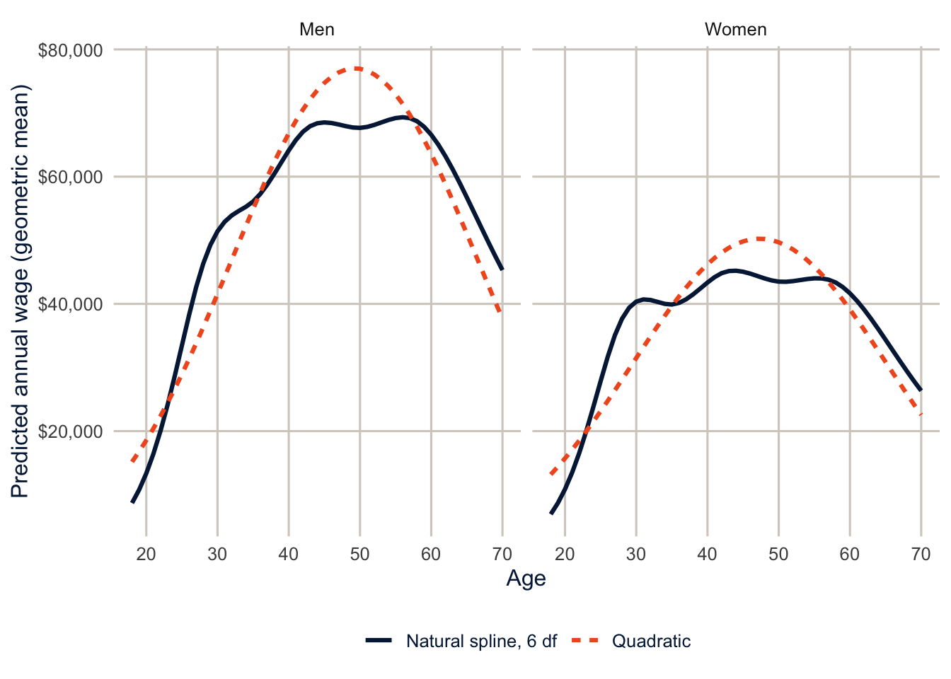
The spline fits much better (its AIC is 3,178 points lower). The quadratic puts men’s peak at age 49, and the spline at 56, with a long plateau. More importantly, the quadratic understates how fast wages grow in the twenties and forces a decline after the peak that’s as steep as the rise before it. For women, the spline shows wages flattening across the early thirties and rising again later, a pattern the quadratic can’t show at all. It’s tempting to read that as what happens to women’s careers when they have young children, and that may be part of it. But this is one year of data, so the curve compares women of different ages, born in different years, who entered the labor market under different conditions; and women who left paid work aren’t in it at all. (Remember from week 7, too, that these are annual wages, so part of any stall is fewer hours worked.)
Summary
Splines let a curve bend where the data bend, with smooth joins at the knots. Natural splines (ns()) behave better than B-splines at the edges of the data, and 4 to 6 degrees of freedom are enough for most demographic curves. Splines are just extra columns in the design matrix, so they work in svyglm() and every other model we’ve used, and you can compare a spline to a straight line with a design-based likelihood ratio test. GAMs choose the amount of smoothing from the data and are excellent for exploring, but mgcv doesn’t do design-based standard errors, so confirm what you find with regression splines in a survey model. Whatever you fit, interpret the curve by predicting from it and plotting, not by reading the coefficients.
Homework 11
Due: April 8, before class.
Which version to do. If you’re in DEM 7283, do the version with your own survey data. If you’re in DEM 5283, do either version, and say at the top of your homework which one you did. If your survey can’t support this week’s method, do the version with my data and say so.
Purpose. Describe nonlinear relationships with curves, choose how flexible the curves should be, and interpret them without overclaiming.
A satisfactory answer shows and interprets predicted curves rather than spline coefficients; says what each curve holds fixed; and doesn’t describe a cross-sectional age pattern as how individuals change as they age.
With your own survey data
Use the full survey design for every estimate unless a step says otherwise, and report each estimate with a standard error or confidence interval.
- Choose an outcome and a continuous predictor (for example, age or income) whose relationship you suspect isn’t a straight line, and state a research question about it.
- Fit a model with the predictor entered as a straight line, and a model with a natural spline
ns(x, df = k)fork= 2, 3, 4 and 6, using the survey design.- Plot the predicted curves on one graph.
- Where do the curves agree, and where do they differ (especially at the extremes of the predictor)?
- How many degrees of freedom would you use, and why?
- Fit a GAM with
mgcv::gam()and a smooth term for the predictor, using rescaled weights as in the chapter.- What effective degrees of freedom does it choose?
- Plot the smooth and compare it with your spline models.
- Does the shape of the curve differ between two groups (for example, by sex or education)? Fit a model that allows it to, show the curves, and interpret the difference.
- Interpret your preferred curve in two or three sentences, and say what it holds fixed. If your predictor is age and your data are cross-sectional, explain why the curve can’t tell you how an individual’s outcome changes as that person ages.
With my data
What is provided. The BRFSS data with age and the design des, the prediction data newdat and the function predict_curve(), and the Texas wage data wages from this chapter.
1. Fit the self-rated health model with ns(age, df = k) for k = 2, 3, 4, 6 and 8, and plot the predicted curves on one graph with predict_curve(). Identify where the curves agree and where they differ, especially at the youngest and oldest ages. How many degrees of freedom would you use, and why? Then explain in two or three sentences why none of these curves can establish how an individual’s health changes as that person ages.
# YOUR CODE HERE2. BMI changes with age too. Fit a survey-weighted linear model for BMI with a natural spline in age interacted with sex, and plot the predicted BMI by age for men and women. Why might average BMI fall at the oldest ages? Think about who is still alive and still answering surveys.
# YOUR CODE HEREOne solution for exercise 2
fit_bmi <- svyglm(bmi ~ ns(age, df = 5) * female, design = des)

nd <- expand_grid(age = 18:80, female = 0:1)
nd |>
  mutate(bmi = as.numeric(predict(fit_bmi, newdata = nd)),
         sex = if_else(female == 1, "Women", "Men")) |>
  ggplot(aes(x = age, y = bmi, colour = sex, linetype = sex)) +
  geom_line(linewidth = 1.1) +
  scale_colour_utsa(palette = "primary") +
  labs(x = "Age", y = "Predicted BMI", colour = NULL, linetype = NULL)
Average BMI rises into middle age and falls after about 60. That’s a cross-sectional pattern, so it mixes at least three things. Part may be aging (people lose muscle and weight late in life), part is selection (people with very high BMI have higher mortality, so they are underrepresented among older survey respondents), and part is cohort (older adults grew up when obesity was much less common). These data can’t separate them.
3. Add a smooth term for BMI, s(bmi), to the GAM for fair or poor health. Plot its predicted effect, holding the other variables fixed. Is the relationship linear? Where is the risk lowest?
# YOUR CODE HERE4. In the wage data, fit ns(AGE, df = 6) separately for workers with and without a bachelor’s degree (EDUC %in% 10:11), and compare the shape of the age-earnings profiles. Where does each group peak?
# YOUR CODE HEREAdditional resources
- Wood (2017), Generalized Additive Models: An Introduction with R, by the author of
mgcv. Thorough, and the reference for anythingmgcvdoes. - Noam Ross’s free course GAMs in R is the gentlest hands-on introduction to
mgcvI know of. - Pedersen, Miller, Simpson and Ross (2019), “Hierarchical Generalized Additive Models”, PeerJ, shows how smooths can vary across groups, which connects this chapter to weeks 12 and 13.
- Harrell (2015), Regression Modeling Strategies, chapter 2, on restricted cubic splines and why they make a better default than polynomials.