library(tidyverse)
library(here)
library(survey)
library(MASS, exclude = "select")
library(pscl)
library(modelsummary)
library(marginaleffects)
library(sparkscolors)

source(here("R", "get_ahrf.R"))
source(here("R", "get_mmsa.R"))
source(here("R", "recode_mmsa.R"))Week 6: Counts and Rates
Introduction
Counts are everywhere in demography. Births, deaths and migrants in a county; the number of children a woman has had; the number of days in the past month someone felt unwell. Before large surveys existed, almost all demography was done this way, on counts of events for places, and the rates we compute from them (birth rates, death rates, migration rates) are still the field’s basic currency.
Counts are non-negative integers, they’re often skewed, and their variance usually grows with their mean, so the linear model fits them badly. This week covers the generalized linear models built for counts, in two settings. The first is rates for places, where the key idea is the offset that turns a model for counts into a model for rates. The second is counts for people, where the key problem is usually too many zeros. Cameron and Trivedi (2013) is the standard reference for everything here.
NoteThis week at a glance
The question. Do counties with more poverty have higher rates of low birth weight births? And how do poor mental health days differ across groups of adults?
By the end of this week you should be able to
- name the event, the denominator (or exposure), the observation period and the unit of analysis for a count;
- explain why a model of event counts across places needs an offset, and interpret an exponentiated coefficient as a rate ratio;
- check a count model for overdispersion, and say what overdispersion tells you about the model.
Before you begin. You need the GLM, the link function and exponentiated coefficients from week 3, and the survey design from week 2. From your demography courses, you need crude and age-specific rates.
Required and optional. Zero-inflated and hurdle models are extensions: read them once you’re comfortable interpreting a basic count model, and use them if your paper has a count outcome with many zeros.
Setup
Demography and places
Macro demography
Before large social surveys arrived in the 1960s, most demographic research was done on aggregates, not individuals, because that’s how the data came. If you look at a text like Keyfitz (1968), all of the examples are national-level calculations. Many countries didn’t have enough data to produce good statistical summaries of their populations at all, which is why the United Nations Population Division’s famous Manual X (1983) gave pragmatic formulas for estimating demographic indicators from the basic inputs usually available in census summaries.
Voss (2007) describes most demography before the 1970s and 1980s as macro demography. Before individual microdata existed, all demography was macro demography, and most of it was spatial, because the data were only available for administrative areas: counties, census tracts, ZIP codes, states and nations. In the macro view, the observations are places or other aggregates of people. Even if you have a count of deaths for a region broken down by age and sex, you still know nothing about the individual decedents beyond those categories. That isn’t a criticism. Data like these are invaluable, and most demographic summaries of individual data aggregate by the same characteristics anyway.
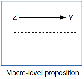
If all we looked at were the individuals in a population, we’d be overwhelmed by the variation, and we wouldn’t be doing statistics anymore, we’d be processing a million anecdotes. The plural of anecdote is not data. Aggregating across basic demographic groups like age and sex is how demographers start to tease apart the differences we care about. If we go further and, data willing, aggregate within places too, we add an extremely important part of human existence: the where of where we live.
Getting data on places
When we talk about data on places, we usually mean some administrative geography, and we often use it as a proxy for the more interesting social spaces we’d really like to study, like neighborhoods and activity spaces. Say I want to study inequality in mortality across neighborhoods in the United States. I immediately hit two hurdles. No national data source puts a sub-city residential location on death certificates, and what is a neighborhood, anyway? I might settle for a single state, because state vital registration systems will sometimes let researchers use the decedent’s address, and a city may maintain its own neighborhood boundaries. But then I run into the “what’s my denominator” problem: there are no official population estimates by age and sex for such small, locally defined areas. This is frustrating. When I advise students on dissertations, there’s often a moment of truth where I lay out the problem of mixing geographic scales and the hard reality of how little data exist for many of the things they want to study.
What usually happens is that we proxy the places we want with places we can get data for. You see this all over the population health literature, where people want to analyze neighborhoods and what they have are census tracts. Tracts aren’t social spaces! They’re arbitrary areas of 3,000 to 5,000 people that change every ten years, drawn so the Census Bureau can count people. Counties have very rich data, but they aren’t neighborhoods or activity spaces either, though they do have some policy-making authority (county health departments, for one) that could be relevant. States are very large, so you lose the ability to put behavior in a fine-scale context, but states make many decisions that affect their residents’ lives, often more than national decisions do. They’ve become popular units of analysis in health research again, largely because states adopted different parts of the Affordable Care Act (Soni et al. 2017; Courtemanche et al. 2019). Whatever the unit, an analysis of places has limitations we have to acknowledge. These are often called ecological analyses, because we’re estimating associations at the macro scale without observing individual outcomes, and the associations don’t necessarily hold for the individuals inside the places.
For U.S. places, a few sources cover most needs:
tigrisdownloads the Census Bureau’s TIGER/Line boundary files (states, counties, tracts, and so on) assfobjects. They hold geography and GEOIDs, not demographic data, but the GEOIDs link them to every federal statistical product.cb = TRUEgets the smaller cartographic boundary files, which are what you want for maps.tidycensus(Walker and Herman, n.d.) uses the Census Bureau’s API to download decennial census, ACS, population estimates, migration flows and PUMS data directly into R, withgeometry = TRUEto attach the boundaries. You’ll need the free API key from week 2.- IPUMS NHGIS (Manson et al., n.d.) has census tables and boundary files for U.S. geographies going back to 1790, which is the place to go for historical work.
- The Area Health Resources File has county data on health care, population and vital events, which we’ll use below.
ACS estimates for small areas come with margins of error, and you should look at them before you map or model anything. The Census Bureau’s MOEs are 90% intervals, so the standard error is the MOE divided by 1.645, and the coefficient of variation is the standard error divided by the estimate. Here’s the share of families below the poverty line in Bexar County tracts. tidycensus looks for your key in the CENSUS_API_KEY environment variable, which census_api_key("your key", install = TRUE) sets up for you.
library(tidycensus)
bexar_pov <- get_acs(geography = "tract", state = "TX", county = "Bexar",
                     variables = "DP03_0119P",   # percent of families below poverty
                     year = 2023, geometry = TRUE, progress_bar = FALSE) |>
  mutate(se = moe / 1.645,
         cv = if_else(estimate > 0, se / estimate, NA_real_),  # CV is undefined at 0
         cv_class = cut(cv, breaks = c(0, 0.15, 0.3, 0.5, Inf),
                        labels = c("Under 0.15", "0.15 to 0.30", "0.30 to 0.50", "Over 0.50")))

ggplot(bexar_pov) +
  geom_sf(aes(fill = cv_class), colour = NA) +
  scale_fill_manual(values = utsa_pal("blues", interpolate = TRUE)(5)[2:5],
                    na.value = utsa_cols("concrete")[[1]],
                    labels = function(x) if_else(is.na(x), "Estimate of 0", x)) +
  labs(fill = "Coefficient of variation") +
  theme_void()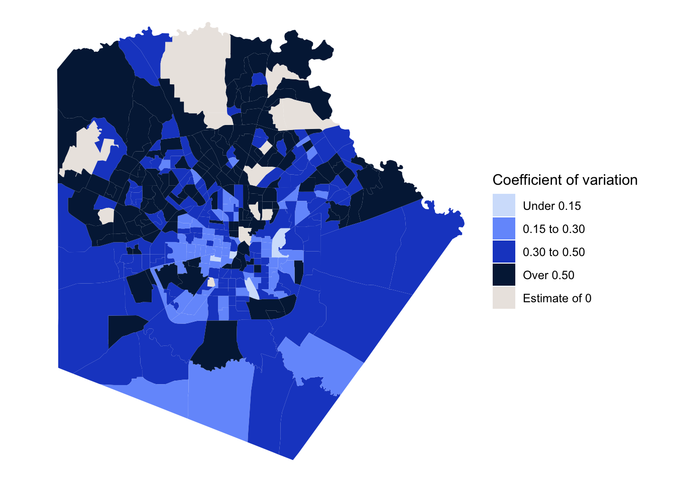
cv_rho  <- cor(bexar_pov$estimate, bexar_pov$cv, method = "spearman", use = "complete.obs")
cv_high <- mean(bexar_pov$cv > 0.3, na.rm = TRUE)
n_zero  <- sum(bexar_pov$estimate == 0, na.rm = TRUE)
The tracts with the least precise estimates are the ones with the lowest poverty rates, because so few sampled families there report incomes below the poverty line. The rank correlation between the poverty rate and its CV is -0.89. A CV above about 0.3 is a common warning sign, and 81% of Bexar County tracts are over it. So a tract map of family poverty is mostly a map of noise, except in the poorest tracts. The 11 tracts with an estimate of zero don’t have a CV at all, but a zero from a sample isn’t a true zero either.
NoteCode explanation: ACS estimates and a map
get_acs()downloads ACS summary estimates: thegeography(tracts here), thestateandcounty, the tablevariables(DP03_0119Pis a “data profile” percent), theyearof the five-year file, andgeometry = TRUEto attach each tract’s boundary. Each row has anestimateand itsmoe.cut(cv, breaks = ..., labels = ...)turns a number into categories, using the break points you give (Infis infinity, so the last class is “anything over 0.5”).geom_sf()draws the boundaries from thegeometrycolumn, filled by a variable, andtheme_void()removes the axes and gridlines, which mean nothing on a map.cor(..., method = "spearman", use = "complete.obs")computes a rank correlation, skipping tracts with a missing value.
Part 1: Rates for places
The data
The Area Health Resources File (AHRF), from the Health Resources and Services Administration, compiles county data on health care, population, and vital events from dozens of federal sources. I’ll model low birth weight births (under 2,500 grams) in U.S. counties, using the three-year totals of births and low birth weight births that the AHRF takes from NCHS natality data. get_ahrf() reads the 2024-2025 file and keeps the variables we need.
ahrf <- get_ahrf() |>
  mutate(rucc = as.integer(na_if(rucc, "")),
         metro = factor(if_else(rucc <= 3, "Metro", "Nonmetro")),
         hpsa = factor(case_when(hpsa == "0" ~ "None",
                                 hpsa == "2" ~ "Part county",
                                 hpsa == "1" ~ "Whole county"),
                       levels = c("None", "Part county", "Whole county")),
         lbw_rate = 1000 * lbw / births,
         suppressed = is.na(lbw) & !is.na(births))
na_if(rucc, "") turns empty text into NA, and as.integer() makes it a number. suppressed is TRUE for counties with a birth count but no low birth weight count (! means “not”). In the summary below, median(births[suppressed]) takes the median of births only for the suppressed counties; the square brackets pick out the elements where the condition is TRUE.
The predictors are the percent of people in poverty, whether the county is metropolitan (rural-urban continuum codes 1 to 3), and whether it is a primary care health professional shortage area (HPSA), in whole or in part.
A problem before we start: suppressed counts
ahrf |>
  filter(!is.na(metro)) |>
  group_by(metro) |>
  summarise(counties = n(),
            n_suppressed = sum(suppressed),
            share_suppressed = mean(suppressed),
            median_births_suppressed = median(births[suppressed]),
            median_births_reported = median(births[!suppressed], na.rm = TRUE))
#> # A tibble: 2 × 6
#> metro counties n_suppressed share_suppressed median_births_suppressed
#> <fct> <int> <int> <dbl> <dbl>
#> 1 Metro 1252 100 0.0799 74.5
#> 2 Nonmetro 1974 696 0.353 64.5
#> # ℹ 1 more variable: median_births_reported <dbl>NCHS doesn’t release counts below 10, so the AHRF has no low birth weight count for 797 counties. They’re missing, not zero, and the difference matters: a zero would say the county had no low birth weight births, while a suppressed count says it had somewhere between 1 and 9 that we aren’t allowed to see. And they aren’t missing at random. Most of them are small nonmetropolitan counties: about a third of nonmetro counties are suppressed, compared with fewer than one in ten metro counties. If we drop them, which is what I do below, the results describe counties with enough births to report, and the comparison between metro and nonmetro counties is a comparison between metro counties and the larger nonmetro counties. I’d name that limitation explicitly in a paper. Pooling more years, or using restricted-use natality files, are the usual ways around it.
ahrf_cc <- ahrf |>
  filter(!is.na(lbw), !is.na(births), !is.na(pov_pct), !is.na(metro), !is.na(hpsa))
nrow(ahrf_cc)
#> [1] 2313Mapping the outcome
When the observations are places, a map is almost a required part of the analysis, and it often says more about the distribution of the outcome than a histogram or a table of summary statistics. tigris gets the county boundaries, and the AHRF’s five-digit FIPS code joins them to the data. I show the suppressed counties in their own color rather than leaving them blank, because where the missing data are is part of the story. I also leave the county borders off, so they don’t swamp the variation, and draw the state borders on top. For a map that will be shown to the public, I’d also add a scale bar and a north arrow (the ggspatial package does both).
options(tigris_use_cache = TRUE)

lower48 <- c("02", "15", "60", "66", "69", "72", "78")
counties_sf <- tigris::counties(cb = TRUE, year = 2023, resolution = "20m",
                                progress_bar = FALSE) |>
  filter(!STATEFP %in% lower48)
states_sf <- tigris::states(cb = TRUE, year = 2023, resolution = "20m",
                            progress_bar = FALSE) |>
  filter(!STATEFP %in% lower48)

lbw_map <- counties_sf |>
  left_join(ahrf, by = c("GEOID" = "fips_st_cnty")) |>
  mutate(lbw_q = cut(lbw_rate,
                     breaks = quantile(lbw_rate, probs = seq(0, 1, 0.2), na.rm = TRUE),
                     include.lowest = TRUE, dig.lab = 3),
         lbw_q = fct_na_value_to_level(lbw_q, "Suppressed"))

ggplot(lbw_map) +
  geom_sf(aes(fill = lbw_q), colour = NA) +
  geom_sf(data = states_sf, fill = NA, colour = "white", linewidth = 0.3) +
  # drop the Limestone end of the ramp so the lowest class stands apart from
  # the Concrete used for suppressed counties
  scale_fill_manual(values = set_names(c(utsa_pal("blues", interpolate = TRUE)(6)[2:6],
                                         utsa_cols("concrete")[[1]]),
                                       levels(lbw_map$lbw_q))) +
  coord_sf(crs = 5070) +
  labs(fill = "LBW per 1,000") +
  theme_void() +
  theme(legend.position = "bottom", text = element_text(colour = utsa_cols("midnight")))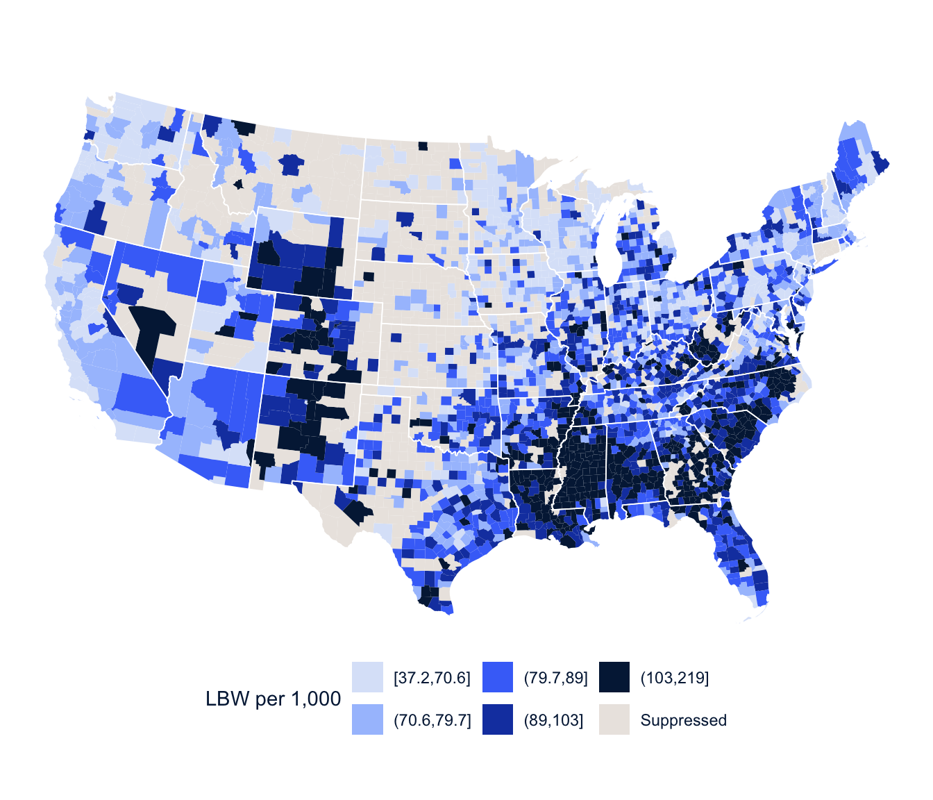
NoteCode explanation: a county map
tigris::counties() and tigris::states() download boundary files; cb = TRUE and resolution = "20m" get simplified versions that draw quickly. filter(!STATEFP %in% lower48) drops Alaska, Hawaii and the territories by their state codes (the vector is named for what’s left). left_join(ahrf, by = c("GEOID" = "fips_st_cnty")) matches the map to the data when the ID columns have different names. quantile(lbw_rate, probs = seq(0, 1, 0.2)) finds the quintile break points, and fct_na_value_to_level() turns the missing (suppressed) counties into a category of their own so they get a color. coord_sf(crs = 5070) draws the map in a projection suited to the lower 48 states.
The highest rates are concentrated in the Southeast, along the lower Mississippi, across the Black Belt of Alabama and Georgia and up into Appalachia, with another cluster in the high-altitude counties of Colorado, Wyoming and New Mexico. And the gray counties make the suppression problem visible: they’re the sparsely populated counties of the Great Plains and the interior West.
A GLM for every outcome
Week 3 introduced the generalized linear model, and here is the bigger picture. The linear model is the GLM with a Normal distribution and the identity link, and glm() with family = gaussian gives exactly the same estimates as lm(). The GLM summary reports the deviance where lm() reports the residual standard error, but for the Gaussian they’re the same information: the deviance is the residual sum of squares, and the square root of the deviance divided by its degrees of freedom is the residual standard error.
Different distributions fit different kinds of outcomes, and each has a usual link function that keeps the linear predictor on the scale of the mean (Nelder and Wedderburn 1972; McCullagh and Nelder 1989):
| Distribution | Mean | Variance | Usual link | Range of outcome |
|---|---|---|---|---|
| Gaussian | \(\mu\) | \(\sigma^2\) | Identity | \((-\infty, \infty)\) |
| Binomial | \(\pi\) | \(n\pi(1 - \pi)\) | \(\log\left(\frac{\pi}{1 - \pi}\right)\) | \(\frac{0, 1, 2, \dots, n}{n}\) |
| Poisson | \(\lambda\) | \(\lambda\) | \(\log(\lambda)\) | \(0, 1, 2, \dots\) |
| Negative binomial | \(\mu\) | \(\mu + \mu^2/\theta\) | \(\log(\mu)\) | \(0, 1, 2, \dots\) |
| Gamma | \(\mu\) | \(\phi\mu^2\) | \(\log(\mu)\) | \((0, \infty)\) |
These aren’t all the possibilities, but they’re the ones you’ll use most, and they’re available in almost any statistics package. The VGAM package (which we used last week) and gamlss add many more.
Rates and offsets
The Poisson model says that the count \(y_i\) in county \(i\) has mean \(\mu_i\), with variance equal to the mean, and models the log of the mean:
\[ \log(\mu_i) = \mathbf{x}_i'\boldsymbol\beta \]
But a county with 50,000 births will have more low birth weight births than a county with 500 for no reason other than its size. Here are three made-up counties:
| County | Births | Low birth weight births | Rate per 1,000 births |
|---|---|---|---|
| A | 500 | 40 | 80 |
| B | 50,000 | 4,000 | 80 |
| C | 200 | 20 | 100 |
A and B have the same rate, but B has 100 times as many low birth weight births, simply because it has 100 times as many births. And C has the fewest events of all, but the highest rate. A count tells us how many events happened; a rate relates the events to the amount of exposure (here, the number of births at risk). A model of the counts alone would mostly describe county size. What we care about is the rate, \(\mu_i / n_i\), where \(n_i\) is the number of births. Taking logs,
\[ \log\left(\frac{\mu_i}{n_i}\right) = \mathbf{x}_i'\boldsymbol\beta \quad\Longleftrightarrow\quad \log(\mu_i) = \log(n_i) + \mathbf{x}_i'\boldsymbol\beta \]
The term \(\log(n_i)\) is the offset. It’s a predictor whose coefficient is fixed at 1, and it turns the count model into a rate model. That’s the difference between an offset and an ordinary predictor. If we put \(\log(n_i)\) in the model as a predictor, the model would estimate its coefficient. We don’t want that, because we already know the relationship: twice the births at risk means, all else equal, twice the expected events. The offset builds that known exposure into the model instead of estimating it. Any model for demographic counts across units of different sizes needs an offset (or a denominator of some kind), and the most common mistake I see in student papers is leaving it out.
So there are really three ways to use the Poisson for places:
- A pure count model, \(\log(\lambda_i) = \mathbf{x}_i'\boldsymbol\beta\), which only makes sense if every place has the same population or area. That almost never happens in demographic data, so you’ll rarely use it.
- A rate model, with the log of the population at risk as the offset. This is the most common way demographic counts are analyzed, and it’s the model above.
- A relative risk model, with the log of an expected count as the offset, which I come back to at the end of Part 1.
Whichever you use, the coefficients are on the log scale, and you exponentiate them to interpret them. If \(\beta_1 = 0.025\), then \(\exp(0.025) = 1.025\). In a pure count model, a one-unit increase in \(x_1\) multiplies the mean count by 1.025, so if the mean is 10 when \(x_1 = 0\), it’s 10.25 when \(x_1 = 1\). In a rate model, the same coefficient multiplies the rate by 1.025, a 2.5% increase.
One practical note: every place needs a population (or expected count) greater than zero, because \(\log(0)\) isn’t a number and glm() will stop with an error. The AHRF counties with suppressed birth counts are already gone from ahrf_cc, so that’s not a problem here.
fit_pois <- glm(lbw ~ offset(log(births)) + pov_pct + metro + hpsa,
                family = poisson, data = ahrf_cc)
summary(fit_pois)
#>
#> Call:
#> glm(formula = lbw ~ offset(log(births)) + pov_pct + metro + hpsa,
#> family = poisson, data = ahrf_cc)
#>
#> Coefficients:
#> Estimate Std. Error z value Pr(>|z|)
#> (Intercept) -2.7287489 0.0079413 -343.616 < 2e-16 ***
#> pov_pct 0.0249708 0.0004254 58.698 < 2e-16 ***
#> metroNonmetro -0.0727025 0.0058325 -12.465 < 2e-16 ***
#> hpsaPart county -0.0421760 0.0078185 -5.394 6.88e-08 ***
#> hpsaWhole county -0.0508765 0.0116346 -4.373 1.23e-05 ***
#> ---
#> Signif. codes: 0 '***' 0.001 '**' 0.01 '*' 0.05 '.' 0.1 ' ' 1
#>
#> (Dispersion parameter for poisson family taken to be 1)
#>
#> Null deviance: 10013.9 on 2312 degrees of freedom
#> Residual deviance: 6515.2 on 2308 degrees of freedom
#> AIC: 19772
#>
#> Number of Fisher Scoring iterations: 4
NoteCode explanation: a Poisson rate model
glm() fits a generalized linear model to ordinary (non-survey) data, the way svyglm() does for survey data. family = poisson makes it a Poisson model with a log link. offset(log(births)) in the formula adds the log of the number of births as an offset, with its coefficient fixed at 1. The summary() coefficients are on the log scale, so exponentiate them (exp(coef(fit_pois))) to get rate ratios.
At the top of the chapter, library(MASS, exclude = "select") loads MASS (for glm.nb(), below) without its select() function, which would otherwise hide dplyr::select(), the package-conflict problem from week 1.
Exponentiated Poisson coefficients are rate ratios. Each percentage point of poverty is associated with a low birth weight rate 2.5% higher, and nonmetro counties have rates 7.0% lower than metro counties with the same poverty and shortage status. The intercept, exponentiated, is the rate in a metro, non-shortage county with zero poverty: 65.3 per 1,000 births.
Here is what happens without the offset:
fit_no_offset <- glm(lbw ~ pov_pct + metro + hpsa, family = poisson, data = ahrf_cc)
round(cbind(with_offset = coef(fit_pois), without_offset = coef(fit_no_offset)), 3)
#> with_offset without_offset
#> (Intercept) -2.729 4.881
#> pov_pct 0.025 0.003
#> metroNonmetro -0.073 -2.044
#> hpsaPart county -0.042 0.776
#> hpsaWhole county -0.051 -0.607Without the offset, the nonmetro coefficient says nonmetro counties have about 87% fewer low birth weight births, which is true and useless: they have fewer births of every kind. The model is describing county size, not risk.
TipReading the result: a right and a wrong interpretation
Right: “Comparing counties with the same metropolitan status and shortage-area status, each additional percentage point of poverty is associated with a low birth weight rate about 2.5% higher.”
Wrong: “Each additional percentage point of poverty causes 2.5% more low birth weight births in a county.” It’s a rate ratio, so it’s about the rate, not the number of births; it compares different counties, not one county getting poorer; and it describes counties, not mothers. A county-level association doesn’t tell you that poorer mothers have more low birth weight babies, which is the ecological problem from the start of the chapter.
Overdispersion
The Poisson assumes the variance equals the mean for places with the same values of the predictors. That’s a statement about the conditional variance: the raw counts across all counties will obviously vary far more than their mean, because counties differ in size and poverty, and that part the model already accounts for. Counts for places still rarely meet the assumption, because counties with the same predictor values differ in many ways the model doesn’t include. A quick check is the Pearson chi-square divided by its degrees of freedom, which should be near 1.
sum(residuals(fit_pois, type = "pearson")^2) / fit_pois$df.residual#> [1] 2.851721residuals(fit_pois, type = "pearson") gives each county’s Pearson residual, its observed minus fitted count divided by the standard deviation the Poisson expects. If the Poisson is right, the squared Pearson residuals average about 1. fit_pois$df.residual is the number of counties minus the number of coefficients.
A dispersion of about 2.9 means the variance is nearly three times what the Poisson assumes, so the Poisson standard errors are too small. If overdispersion is present and we ignore it, we can call a relationship significant when it isn’t.
The residual deviance gives a formal goodness-of-fit test, because if the model is right it has a \(\chi^2\) distribution with the residual degrees of freedom (\(n - p\)):
c(deviance = deviance(fit_pois), df = df.residual(fit_pois),
  p = pchisq(deviance(fit_pois), df.residual(fit_pois), lower.tail = FALSE))
#> deviance df p
#> 6515.185 2308.000 0.000A p-value of essentially zero says the Poisson doesn’t fit these data. (If the p-value were above 0.05, we couldn’t reject the hypothesis that it does.)
Treat overdispersion as a clue before you treat it as a nuisance. It says the counties vary more than the model explains, and it’s worth asking why. Is an important predictor missing (the racial composition of the county, say, which is strongly associated with low birth weight)? Are a few unusual counties driving it? Are neighboring counties more alike than the model assumes? Fixing any of those can reduce the overdispersion and improve the model’s coefficients, not just their standard errors. Once you’ve done what you can, some extra variation almost always remains, and there are two common ways to account for it.
The quasi-Poisson model keeps the Poisson estimates and adds a dispersion parameter, so that \(\text{Var}(y_i) = \phi\lambda_i\) instead of \(\lambda_i\). In the Poisson, \(\phi\) is fixed at 1, and in the quasi-Poisson it’s estimated, which multiplies every standard error by \(\sqrt{\phi}\). The negative binomial model adds a parameter that lets the variance grow faster than the mean. It’s a real likelihood, so it can be compared with the Poisson by AIC, and its estimates differ a little from the Poisson’s because it weights the counties differently.
The negative binomial comes in two common forms. The NB1 model lets the variance grow linearly with the mean, and the NB2 model, the one most software fits, lets it grow with the square of the mean:
\[ \text{NB1: } \text{Var}(y_i) = \lambda_i + \theta\lambda_i \qquad\qquad \text{NB2: } \text{Var}(y_i) = \lambda_i + \lambda_i^2/\theta \]
MASS::glm.nb() fits NB2. (NB1 looks a lot like the quasi-Poisson, but it’s a full likelihood.) glmmTMB fits both, with family = nbinom1 and nbinom2, and gamlss fits both along with a long list of other distributions, and lets you model the variance as well as the mean.
fit_qp <- glm(lbw ~ offset(log(births)) + pov_pct + metro + hpsa,
              family = quasipoisson, data = ahrf_cc)
fit_nb <- glm.nb(lbw ~ offset(log(births)) + pov_pct + metro + hpsa, data = ahrf_cc)

modelsummary(list("Poisson" = fit_pois, "Quasi-Poisson" = fit_qp,
                  "Negative binomial" = fit_nb),
             exponentiate = TRUE, fmt = 3,
             statistic = "({std.error})",
             gof_map = c("nobs", "aic"),
title = "Rate ratios for low birth weight, U.S. counties")| Poisson | Quasi-Poisson | Negative binomial | |
|---|---|---|---|
| (Intercept) | 0.065 | 0.065 | 0.062 |
| (0.001) | (0.001) | (0.001) | |
| pov_pct | 1.025 | 1.025 | 1.028 |
| (0.000) | (0.001) | (0.001) | |
| metroNonmetro | 0.930 | 0.930 | 0.922 |
| (0.005) | (0.009) | (0.008) | |
| hpsaPart county | 0.959 | 0.959 | 0.967 |
| (0.007) | (0.013) | (0.014) | |
| hpsaWhole county | 0.950 | 0.950 | 0.971 |
| (0.011) | (0.019) | (0.018) | |
| Num.Obs. | 2313 | 2313 | 2313 |
| AIC | 19772.4 | 16830.7 |
AIC(fit_pois, fit_nb)#> df AIC
#> fit_pois 5 19772.39
#> fit_nb 6 16830.69glm.nb() (from MASS) fits the negative binomial model; it takes the same formula as glm() and always uses a log link. family = quasipoisson fits the quasi-Poisson. In modelsummary(), statistic = "({std.error})" puts the standard error in parentheses under each estimate, and gof_map = c("nobs", "aic") shows the number of observations and the AIC.
The negative binomial fits far better by AIC. The poverty rate ratio is a bit larger, and the shortage area effects, which looked clearly significant in the Poisson, are much less certain once the extra variation is accounted for. That is the general pattern: an overdispersed Poisson overstates how much you know.
The quasi-Poisson’s coefficients are identical to the Poisson’s, and its standard errors are not. Form the ratio of the two sets of standard errors and it’s the same for every coefficient:
se_ratio <- sqrt(diag(vcov(fit_qp))) / sqrt(diag(vcov(fit_pois)))
round(se_ratio, 3)
#> (Intercept) pov_pct metroNonmetro hpsaPart county
#> 1.689 1.689 1.689 1.689
#> hpsaWhole county
#> 1.689sqrt(summary(fit_qp)$dispersion)#> [1] 1.688704Every ratio is exactly \(\sqrt{\phi}\), the square root of the quasi-Poisson dispersion, and \(\phi\) is the same Pearson dispersion we computed above. That’s all the quasi-Poisson does. It’s a quick fix, but because it’s fit by quasi-likelihood, it has no AIC and can’t be compared with other models that way. Breslow (1984) proposed a model that adds an extra-Poisson variance parameter and is fit by reweighted maximum likelihood, so each coefficient’s standard error gets its own adjustment instead of one common factor, and the dispmod package implements it.
The binomial alternative
Low birth weight births are a subset of births, so a binomial model for the proportion is also natural. glm() takes the outcome as the number of successes and failures:
fit_bin <- glm(cbind(lbw, births - lbw) ~ pov_pct + metro + hpsa,
               family = binomial, data = ahrf_cc)
round(cbind(poisson = coef(fit_pois), binomial = coef(fit_bin)), 3)
#> poisson binomial
#> (Intercept) -2.729 -2.666
#> pov_pct 0.025 0.027
#> metroNonmetro -0.073 -0.080
#> hpsaPart county -0.042 -0.047
#> hpsaWhole county -0.051 -0.056cbind(lbw, births - lbw) gives glm() two columns: the number of “successes” (low birth weight births) and “failures” (all other births) in each county.
The coefficients are close, because when an outcome is uncommon (about 9% of births here), the odds and the rate are nearly the same thing. For common outcomes they diverge.
So which denominator is which? Use the binomial when the denominator is a fixed number of trials, each of which can produce the event at most once: births that might be low birth weight, women who might have had a birth this year, people who might have died. The count can’t exceed the denominator. Use a rate model (Poisson or negative binomial with an offset) when the denominator is person-time or another measure of exposure, and events could in principle happen more than once per unit: hospitalizations per 1,000 person-years, or deaths per person-years lived when people enter and leave the population during the year. For an uncommon event counted over a fixed population, the two give nearly the same answer, as here.
With the count-based binomial, the odds ratio interpretation is less natural than it is for individuals, and when I interpret these coefficients I describe them as approximate percent changes in the rate. The poverty coefficient exponentiates to 1.028, so the odds of a low birth weight birth are 2.8% higher for every percentage point of poverty. predictions() shows what that means for the rate itself, for two counties that differ by one point of poverty:
bin_pred <- predictions(fit_bin, newdata = datagrid(pov_pct = c(15, 16), metro = "Metro",
                                                    hpsa = "None"))
bin_pred[, c("pov_pct", "estimate")]
#>
#> Estimate
#> 0.0951
#> 0.0975bin_pred$estimate[2] / bin_pred$estimate[1] - 1#> [1] 0.02515995The rate rises by 2.52%, a little less than the odds. With an outcome this uncommon the two are close, which is why reading the odds ratio as a percent change in the rate is a reasonable shorthand here, and why it stops being reasonable as the outcome gets more common.
The beta distribution is another option for proportions. It lives between 0 and 1, like the binomial’s \(\pi\), but it has its own precision parameter, so it sidesteps the overdispersion that so often plagues the binomial. betareg fits it (Cribari-Neto and Zeileis 2010), with the same logit, probit or complementary log-log links, and a second formula after | models the precision too. It works on the observed proportions, so it doesn’t know that a rate based on 20 births is less reliable than one based on 20,000, which is a real disadvantage for county data like these.
library(betareg)
fit_beta <- betareg(I(lbw / births) ~ pov_pct + metro + hpsa, data = ahrf_cc)
fit_beta_disp <- betareg(I(lbw / births) ~ pov_pct + metro + hpsa | metro, data = ahrf_cc)
AIC(fit_beta, fit_beta_disp)
Age standardization in a regression model
The binomial and the Poisson also give us a regression version of age standardization. Crude death rates mix two things: how likely people are to die at each age, and how many people there are at each age. To compare places fairly, we need to hold the age structure constant. I’ll use deaths and population by age for Texas and California in 2016, from the CDC WONDER Compressed Mortality File.
age_levels <- c("< 1 year", "1-4 years", "5-9 years", "10-14 years", "15-19 years",
                "20-24 years", "25-34 years", "35-44 years", "45-54 years",
                "55-64 years", "65-74 years", "75-84 years", "85+ years")

txca <- read_tsv(here("data", "CMF_TX_CA_age.txt"), na = c("", "Not Applicable", "Suppressed"),
                 show_col_types = FALSE) |>
  rename(state = State, age = `Age Group`, deaths = Deaths, population = Population) |>
  filter(age != "Not Stated") |>
  mutate(age = factor(age, levels = age_levels),
         state = factor(state, levels = c("California", "Texas")),
         deaths = as.numeric(deaths), population = as.numeric(population)) |>
  select(state, age, deaths, population)

txca |>
  group_by(state) |>
  summarise(deaths = sum(deaths), population = sum(population)) |>
  mutate(crude_rate = 1e5 * deaths / population)
#> # A tibble: 2 × 4
#> state deaths population crude_rate
#> <fct> <dbl> <dbl> <dbl>
#> 1 California 262215 39250017 668.
#> 2 Texas 191962 27862596 689.txca |>
group_by(state) |>
mutate(share = population / sum(population)) |>
ggplot(aes(x = age, y = share, colour = state, linetype = state, group = state)) +
geom_line(linewidth = 1.2) +
geom_point(size = 2) +
scale_colour_utsa(palette = "primary") +
scale_y_continuous(labels = scales::label_percent()) +
labs(x = "Age group", y = "Share of population", colour = NULL, linetype = NULL) +
theme(axis.text.x = element_text(angle = 45, hjust = 1))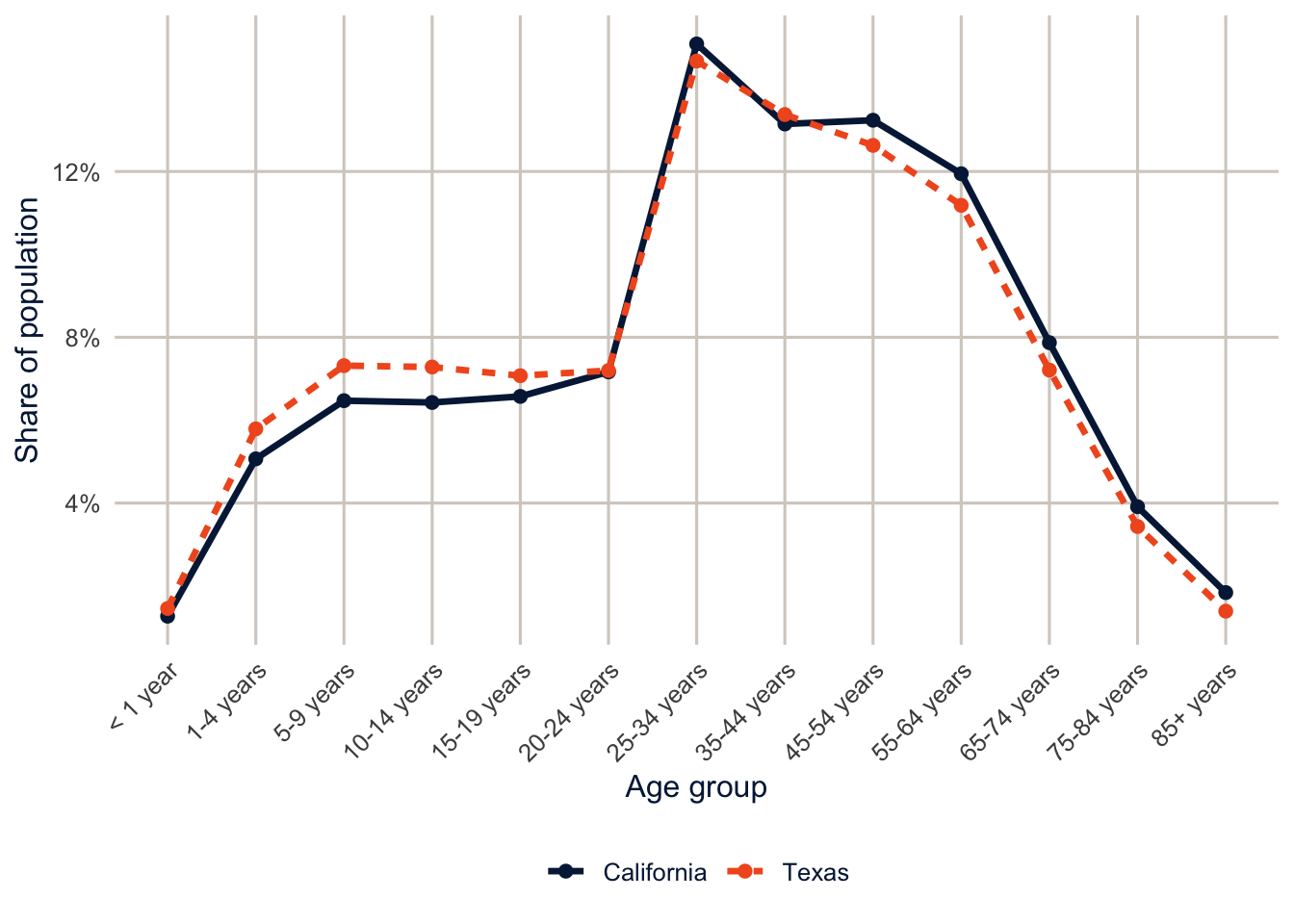
read_tsv() reads a tab-separated text file, rename() gives the columns shorter names (new = old), and the na argument says which entries mean “missing.”
Texas has a younger population than California, so its crude death rate understates its mortality relative to California’s. That’s the whole reason for standardizing: a fair comparison between two populations should compare the risk of death at each age, not the accident of how many people each state happens to have at old ages. To standardize in the regression framework, we put age in the model. The state coefficient is then the difference between the states holding the age structure constant, which is the difference in age-standardized rates.
fit_txca_bin <- glm(cbind(deaths, population - deaths) ~ age + state,
                    family = binomial, data = txca)
fit_txca_pois <- glm(deaths ~ offset(log(population)) + age + state,
                     family = poisson, data = txca)
fit_txca_crude <- glm(deaths ~ offset(log(population)) + state,
                      family = poisson, data = txca)

exp(c(crude = coef(fit_txca_crude)[["stateTexas"]],
      binomial = coef(fit_txca_bin)[["stateTexas"]],
      poisson = coef(fit_txca_pois)[["stateTexas"]]))
#> crude binomial poisson
#> 1.031279 1.198538 1.187149Without age in the model, Texas’s death rate looks only 3.1% higher than California’s. After standardizing for age, Texas has a mortality rate 18.7% higher, and the binomial and Poisson models agree almost exactly. This is a model-based relative of the direct and indirect standardization you’ve done by hand, and next week’s Kitagawa decomposition will split a crude difference like this one into the part due to rates and the part due to composition.
Expected counts and standardized ratios
Epidemiologists often use the expected count as the offset instead of the population. The expected count is what a county would have if it had the overall rate: \(E_i = n_i \times \sum_j y_j / \sum_j n_j\). This is internal standardization, and the ratio \(y_i / E_i\) is the standardized incidence ratio (SIR).
overall_rate <- sum(ahrf_cc$lbw) / sum(ahrf_cc$births)

ahrf_cc <- ahrf_cc |>
  mutate(expected = births * overall_rate,
         sir = lbw / expected)

fit_sir <- glm.nb(lbw ~ offset(log(expected)) + pov_pct + metro + hpsa, data = ahrf_cc)
round(cbind(births_offset = coef(fit_nb), expected_offset = coef(fit_sir)), 4)
#> births_offset expected_offset
#> (Intercept) -2.7766 -0.3217
#> pov_pct 0.0280 0.0280
#> metroNonmetro -0.0816 -0.0816
#> hpsaPart county -0.0335 -0.0335
#> hpsaWhole county -0.0299 -0.0299Only the intercept changes, because \(\log(E_i) = \log(n_i) + \log(\text{overall rate})\), and the constant moves into the intercept. Choosing between these offsets is about what the intercept and the fitted values mean, not about the covariate effects. With age-specific rates in the expected count (indirect standardization), the SIR also adjusts for age, which is the usual reason to use it for mortality.
Here’s that for Texas and California. The naive expected count uses the crude death rate of both states combined. The age-specific version applies each age group’s combined death rate to each state’s population in that age group.
txca <- txca |>
  mutate(e_crude = population * sum(deaths) / sum(population)) |>
  group_by(age) |>
  mutate(e_age = population * sum(deaths) / sum(population)) |>
  ungroup()

txca |>
  group_by(state) |>
  summarise(observed = sum(deaths), expected_crude = sum(e_crude),
            expected_age = sum(e_age)) |>
  mutate(smr_age = observed / expected_age)
#> # A tibble: 2 × 5
#> state observed expected_crude expected_age smr_age
#> <fct> <dbl> <dbl> <dbl> <dbl>
#> 1 California 262215 265620. 280889. 0.934
#> 2 Texas 191962 188557. 173288. 1.11fit_rr <- glm(deaths ~ offset(log(e_age)) + age + state, family = poisson, data = txca)
exp(coef(fit_rr)[["stateTexas"]])#> [1] 1.187149Summed over age, the expected counts based on the crude rate look closer to the observed deaths, but that’s an illusion. They ignore age, so they credit California’s older population with too few expected deaths and Texas’s younger population with too many. Once the expected counts use age-specific rates, Texas has 10.8% more deaths than its age structure would predict, and California has 6.6% fewer. In the model with age-specific expected counts, the Texas rate ratio is identical to the one from the rate model, even though the offset is different. Different denominators, same comparison.
ahrf_cc |>
  ggplot(aes(x = pov_pct, y = sir, size = births)) +
  geom_hline(yintercept = 1, colour = utsa_cols("smoke"), linewidth = 1) +
  geom_point(alpha = 0.4, colour = utsa_cols("midnight")) +
  geom_smooth(aes(weight = births), method = "loess", se = FALSE,
              colour = utsa_cols("orange"), linewidth = 1.2, show.legend = FALSE) +
  scale_size_area(max_size = 6, guide = "none") +
  labs(x = "Percent of persons in poverty", y = "Standardized incidence ratio")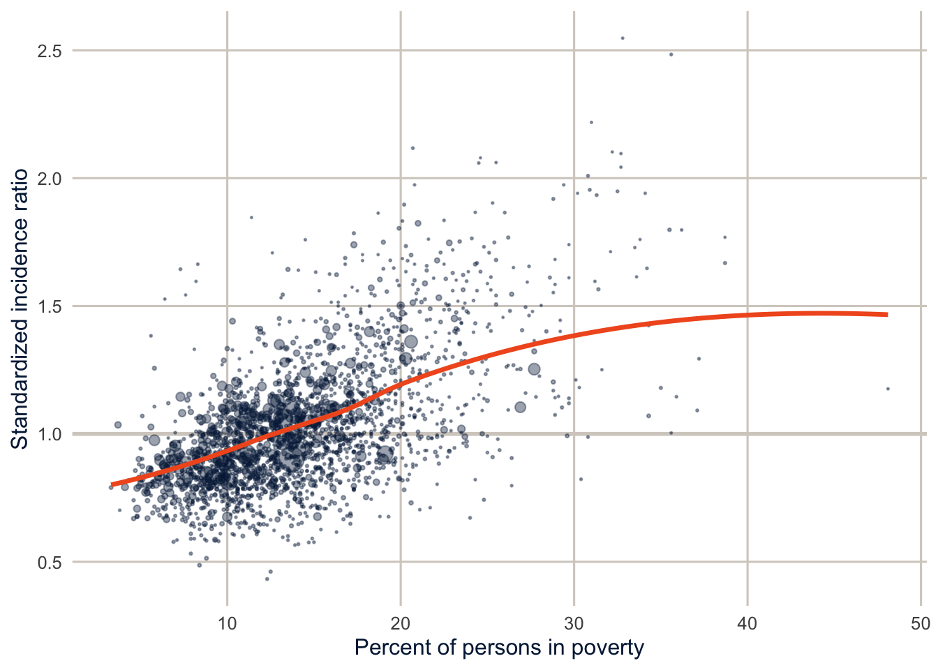
Part 2: Counts for people
Poor mental health days
The BRFSS asks, “Now thinking about your mental health, which includes stress, depression, and problems with emotions, for how many days during the past 30 days was your mental health not good?” recode_mmsa() turns the answers into ment_days, from 0 to 30.
brfss <- get_mmsa(2024) |>
  recode_mmsa() |>
  mutate(complete = complete.cases(ment_days, agec, female, educ, race_eth, income))

des <- svydesign(ids = ~1, strata = ~ststr, weights = ~mmsawt, data = brfss)svytable(~ment_days, des) |>
as_tibble() |>
mutate(ment_days = as.integer(ment_days),
share = n / sum(n)) |>
ggplot(aes(x = ment_days, y = share)) +
geom_col(fill = utsa_cols("midnight")) +
scale_y_continuous(labels = scales::label_percent()) +
labs(x = "Days of poor mental health, past 30 days", y = "Share of adults")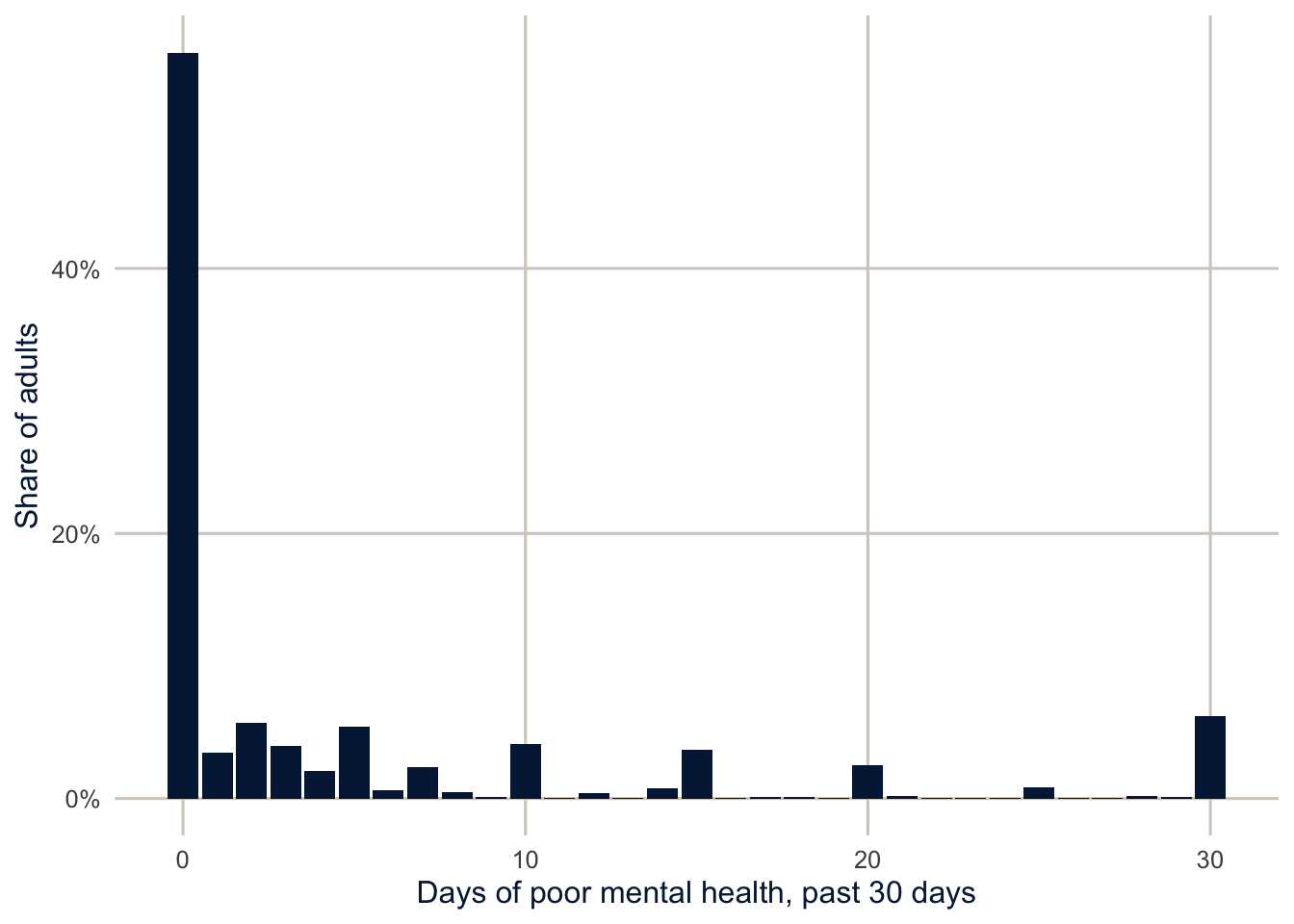
This is a very typical count distribution for a survey question. About 56% of adults report no poor mental health days, the rest are spread out with a long tail, and there are spikes at 5, 10, 15, 20 and 30, because people round. The spike at 30 is also a ceiling: “every day” is as high as the question goes. The weighted mean is 4.8 days.
A population-average model
If what we want is the mean number of days in the population, and how it differs across groups, a Poisson-type model fit with svyglm() does the job. The quasipoisson family gives the same point estimates as the Poisson and lets the design-based standard errors handle the overdispersion.
fit_svy <- svyglm(ment_days ~ agec + female + educ + race_eth + income,
                  design = subset(des, complete), family = quasipoisson())

modelsummary(list("Survey quasi-Poisson" = fit_svy), exponentiate = TRUE,
             fmt = 3, gof_map = "nobs",
title = "Rate ratios for poor mental health days")| Survey quasi-Poisson | |
|---|---|
| (Intercept) | 9.035 |
| (0.420) | |
| agec25-34 | 0.998 |
| (0.029) | |
| agec35-44 | 0.911 |
| (0.027) | |
| agec45-54 | 0.781 |
| (0.025) | |
| agec55-64 | 0.656 |
| (0.021) | |
| agec65+ | 0.390 |
| (0.013) | |
| female | 1.304 |
| (0.023) | |
| educHS graduate | 1.048 |
| (0.043) | |
| educSome college | 1.128 |
| (0.047) | |
| educCollege graduate | 0.890 |
| (0.038) | |
| race_ethNH Black | 0.882 |
| (0.022) | |
| race_ethNH Other | 0.792 |
| (0.031) | |
| race_ethNH Multiracial | 1.160 |
| (0.046) | |
| race_ethHispanic | 0.709 |
| (0.021) | |
| income$25k-$50k | 0.767 |
| (0.021) | |
| income$50k-$100k | 0.656 |
| (0.019) | |
| income$100k+ | 0.513 |
| (0.016) | |
| Num.Obs. | 180351 |
svytable(~ment_days, des) in the figure above counts the weighted number of adults at each number of days. The model uses quasipoisson() with the design, as described.
Two things are worth being clear about. First, the model is for the mean number of days, and that’s all it claims to get right. The days are bounded at 30, and a Poisson distribution would put some probability above 30, but that doesn’t matter for estimating how the mean differs across groups. It would matter if we wanted to predict the whole distribution of days, which is where the next section goes. Second, there’s no offset here, because everyone has the same exposure: 30 days.
The rate ratios read like the county model: adults 65 and older report 61% fewer poor mental health days than adults 18 to 24, and adults with household incomes of $100,000 or more report 49% fewer than those under $25,000. For many questions this is the model I’d report, because it answers a population question with design-based inference.
Where do the zeros come from? (optional)
Sometimes the zeros themselves are the interesting part. A zero can mean two different things: someone whose mental health was fine this month but who has bad stretches, or someone who basically never has poor mental health days. Two families of models take this seriously (Zeileis et al. 2008).
Zero-inflated models (Lambert 1992) say that there are two kinds of people: “structural” zeros, who can only report 0, and everyone else, whose counts follow a Poisson or negative binomial that can also produce zeros. A logit models membership in the structural zero group, and a count model handles the rest.
Hurdle models (Mullahy 1986) say that there’s one process for whether you have any days at all (crossing the hurdle), and a second process, a count model truncated at zero, for how many days you have once you’ve crossed it.
The difference is subtle but real. In a zero-inflated model, zeros come from both parts. In a hurdle model, all zeros come from the first part, and the count part only describes people with at least one day. I find hurdle models easier to explain, because each part answers a plain question: who has any poor mental health days, and among them, how many?
Fitting and comparing the models (optional)
pscl fits both. It takes weights but not a survey design, so I pass the survey weights scaled to average 1. The point estimates then describe the population, but the standard errors treat the data as a simple random sample, so they’re too small, and a large sample doesn’t fix that. I wouldn’t report these standard errors in a paper without fixing them (with replicate weights, as in week 2).
cc <- brfss |>
  filter(complete) |>
  mutate(w = mmsawt / mean(mmsawt))

f_counts <- ment_days ~ agec + female + educ + race_eth + income

fit_p <- glm(f_counts, family = poisson, data = cc, weights = w)
fit_n <- glm.nb(f_counts, data = cc, weights = w)
# two-part formulas: count model | zero (or hurdle) model
f_two <- ment_days ~ agec + female + educ + race_eth + income |
  agec + female + educ + race_eth + income

fit_zinb <- zeroinfl(f_two, dist = "negbin", data = cc, weights = w)
fit_hnb <- hurdle(f_two, dist = "negbin", data = cc, weights = w)
NoteCode explanation: two-part count models
zeroinfl() and hurdle() take a two-part formula: the predictors before the | are for the count part, and the ones after it are for the zero part. Here both parts have the same predictors. dist = "negbin" makes the count part negative binomial. mmsawt / mean(mmsawt) rescales the weights so they average 1, which keeps the estimates the same as with the original weights but stops pscl from treating the sample as if it were the size of the population.
Since the weighted likelihoods aren’t true likelihoods, I won’t compare these models by AIC. A more useful check is whether each model reproduces the distribution of the outcome. For each model, I average the predicted probability of every count from 0 to 30 and compare it with the observed distribution.
counts <- 0:30
wmean <- function(p) colSums(p * cc$w) / sum(cc$w)

freq <- tibble(
  days = counts,
  Observed = map_dbl(counts, \(k) weighted.mean(cc$ment_days == k, cc$w)),
  Poisson = wmean(sapply(counts, \(k) dpois(k, fitted(fit_p)))),
  `Negative binomial` = wmean(sapply(counts, \(k) dnbinom(k, mu = fitted(fit_n),
                                                         size = fit_n$theta))),
  `Zero-inflated NB` = wmean(predict(fit_zinb, type = "prob", at = counts)),
  `Hurdle NB` = wmean(predict(fit_hnb, type = "prob", at = counts))
)

freq |>
  filter(days %in% c(0, 1, 2, 5, 10, 15, 20, 30)) |>
knitr::kable(digits = 3)| days | Observed | Poisson | Negative binomial | Zero-inflated NB | Hurdle NB |
|---|---|---|---|---|---|
| 0 | 0.546 | 0.029 | 0.521 | 0.547 | 0.546 |
| 1 | 0.036 | 0.079 | 0.105 | 0.048 | 0.046 |
| 2 | 0.060 | 0.122 | 0.060 | 0.041 | 0.041 |
| 5 | 0.059 | 0.125 | 0.026 | 0.028 | 0.029 |
| 10 | 0.043 | 0.028 | 0.012 | 0.017 | 0.017 |
| 15 | 0.038 | 0.003 | 0.007 | 0.010 | 0.010 |
| 20 | 0.026 | 0.000 | 0.004 | 0.006 | 0.006 |
| 30 | 0.062 | 0.000 | 0.002 | 0.002 | 0.002 |
For each model, this computes the share of people it expects at each count from 0 to 30. dpois(k, mu) is the Poisson probability of exactly k days for someone with mean mu, and dnbinom() is the negative binomial version; fitted() gives each person’s predicted mean. sapply() runs the calculation for each k and returns a matrix with one column per count, and wmean() takes the weighted average of each column. For the two-part models, predict(..., type = "prob", at = counts) returns those probabilities directly.
freq_long <- freq |>
  pivot_longer(-c(days, Observed), names_to = "model", values_to = "predicted") |>
  mutate(model = fct_inorder(model))

ggplot(freq, aes(x = days)) +
  geom_col(aes(y = Observed), fill = utsa_cols("concrete")) +
  geom_line(data = freq_long, aes(y = predicted, colour = model, linetype = model),
            linewidth = 1.3) +
  geom_point(data = freq_long, aes(y = predicted, colour = model, shape = model),
             size = 1.8) +
  scale_colour_utsa() +
  scale_y_sqrt(labels = scales::label_percent()) +
  labs(x = "Days of poor mental health", y = "Share (square root scale)",
       colour = NULL, linetype = NULL, shape = NULL)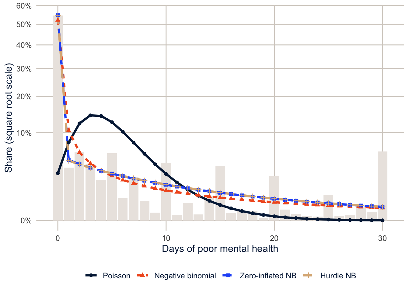
The Poisson is hopeless: it predicts that only 2.9% of adults would report zero days, against 54.6% observed. The negative binomial gets much closer (52.1%), which is a reminder that “too many zeros” is often just overdispersion, and a negative binomial may be all you need. The zero-inflated and hurdle models match the zeros almost exactly. The hurdle model matches them by construction, since its first part is a logit for zero versus not.
But look at the other end of the distribution, because none of the models gets it right. 14.3% of adults report 15 or more poor mental health days, and even the hurdle model predicts only 8.6%. The spike at 30 is the worst of it. The negative binomial family expects a long, thinning tail, and these data have a second mode at the ceiling, made up of people whose mental health was poor every day, or nearly so. The heaping at 5, 10 and 15 is a smaller version of the same problem, since nothing in a count distribution knows that people round. So the zero-inflated and hurdle models fix the zeros and leave a real misfit in the tail. That’s worth knowing before you interpret their count-part coefficients too literally, and it’s a good reason to try a model built for a bounded outcome (see the note at the end of this section).
Interpreting the hurdle model (optional)
show_terms <- c("agec65+", "female", "educCollege graduate", "race_ethHispanic",
                "income$100k+")

tibble(term = show_terms,
       `Any days (odds ratio)` = exp(coef(fit_hnb, model = "zero")[show_terms]),
       `Number of days (rate ratio)` = exp(coef(fit_hnb, model = "count")[show_terms])) |>
knitr::kable(digits = 2)| term | Any days (odds ratio) | Number of days (rate ratio) |
|---|---|---|
| agec65+ | 0.16 | 1.01 |
| female | 1.65 | 1.03 |
| educCollege graduate | 1.25 | 0.76 |
| race_ethHispanic | 0.59 | 0.99 |
| income$100k+ | 0.64 | 0.62 |
Here is where the two parts earn their keep. Look at college graduates, compared with adults who didn’t finish high school. In the zero part, which models the odds of reporting any poor mental health days, the odds ratio is 1.25: college graduates are more likely to report at least one bad day. In the count part, among people with at least one day, college graduates report 24% fewer days. The population-average model from earlier mixes these two opposite patterns into a single rate ratio of 0.89, which hides both. Whether the first pattern is about mental health or about how people with more education answer survey questions about it is a good question, and exactly the kind of thing the model can’t settle for you.
Note
Because the outcome can’t exceed 30, a model for “days out of 30” is a natural alternative. The plain binomial will be badly overdispersed, but the beta-binomial allows for people who are mostly at one end or the other, which is exactly the U shape these data have. glmmTMB(cbind(ment_days, 30 - ment_days) ~ ..., family = betabinomial) fits it, and comparing its predicted distribution with the ones above is a good project.
Homework 6
Due: March 4, before class.
Which version to do. If you’re in DEM 7283, do the version with your own survey data. If you’re in DEM 5283, do either version, and say at the top of your homework which one you did. If your survey can’t support this week’s method, do the version with my data and say so.
Purpose. Model counts and rates with the right denominator, and interpret the results as rates.
A satisfactory answer identifies the event, denominator or exposure, period and unit for each model; interprets exponentiated coefficients as rate ratios in a full sentence; says whether the model respects the outcome’s limits; and describes county-level results as associations for counties, not for individuals.
With your own survey data
Use the full survey design for every estimate unless a step says otherwise, and report each estimate with a standard error or confidence interval.
- Define a count outcome for your data (for example, the number of days of poor health, the number of children ever born, or the number of doctor visits).
- State a research question about your outcome.
- Describe its distribution: the mean, the variance, the share of zeros, and any heaping or ceiling.
- Is an offset term necessary? Why or why not? If it is, what is the exposure?
- Consider a Poisson regression model for the outcome.
- Evaluate the level of dispersion in the outcome.
- Is the Poisson model a good choice?
- Fit a population-average model with
svyglm()andfamily = quasipoisson, and interpret the exponentiated coefficients for your key predictor as rate ratios in full sentences. - Fit a negative binomial model with
glm.nb(), using rescaled weights as in the chapter. - Fit a zero-inflated or hurdle negative binomial model.
- Compare how well the Poisson, negative binomial and zero-inflated or hurdle models reproduce the observed distribution of your outcome, especially the share of zeros and the upper tail.
- Why don’t we compare these weighted models by AIC?
- Which model would you use for your research question, and why?
With my data
What is provided. The AHRF county data (ahrf_cc, with suppressed counties removed) and the models from Part 1; the BRFSS data and design from Part 2.
1. For the low birth weight model in this chapter, identify (a) the event being counted, (b) the denominator, (c) the period it’s counted over, and (d) the unit of analysis, and explain in a sentence why log(births) is an offset rather than a predictor. Then fit a negative binomial model that adds the number of general OB-GYNs per 10,000 population (from obgyn and popn_est_23). Interpret its exponentiated coefficient as a rate ratio, explain why you might expect this association to be confounded by county size even with the offset, and say whether the model respects the limits of the outcome (a low birth weight count can’t exceed the number of births).
# YOUR CODE HERE2. The AHRF also has three-year totals of deaths (deth_3yr_avg_23) and population estimates. Modify get_ahrf() (or read the file directly) to get them, and fit a model for county crude death rates with a population offset. Then explain, in two or three sentences, why a model for crude death rates across counties without age standardization is hard to interpret.
# YOUR CODE HEREA hint for exercise 2
Copy get_ahrf() to your own project, add deaths = deth_3yr_avg_23 to the select(), and change the cache file name so you don’t overwrite the course copy. For the second part, think about what the share of the population over 65 does to a county’s crude death rate.
3. Fit a survey-weighted quasi-Poisson model for poor physical health days (phys_days) with the same predictors as the mental health model. Compare the rate ratios with the mental health model. Which predictors differ most?
# YOUR CODE HERE4. (Optional.) Fit a zero-inflated negative binomial model and a hurdle negative binomial model for phys_days. Compare their predicted distributions with the observed distribution, as in this document, and interpret the education coefficients from both parts of the hurdle model.
# YOUR CODE HEREAdditional resources
- Cameron and Trivedi (2013) is the standard reference for count models, from the Poisson through hurdles and zero inflation.
- Zeileis et al. (2008), “Regression Models for Count Data in R”, Journal of Statistical Software, walks through the Poisson, negative binomial, hurdle and zero-inflated models in R with one running example.
- Preston et al. (2001), Demography: Measuring and Modeling Population Processes, chapters 1 and 2, for rates, person-years and standardization done by hand.