library(tidyverse)
library(here)
library(survey)
library(svyVGAM)
library(marginaleffects)
library(sparkscolors)

source(here("R", "get_mmsa.R"))
source(here("R", "recode_mmsa.R"))
source(here("R", "get_dhs_model.R"))Week 5: Ordinal and Multinomial Logit Models
Introduction
The binary logit is flexible, because almost anything can be squeezed into a yes or no. But squeezing throws information away. Self-rated health has five ordered categories, and collapsing them into “fair or poor” versus everything else treats a move from excellent to good the same as no move at all. The same is true of a political scale that runs from very liberal to very conservative, or a question with “strongly agree” through “strongly disagree.” Other outcomes have categories with no order at all: which method of contraception a woman uses, which of several labor markets a migrant moves to, how a family arranges child care, how someone gets to work. Demographers sometimes call these alternative decision-making processes, because the person (in principle) chooses one option from a set.
Before choosing a model, decide what kind of outcome you have. Try classifying these yourself before reading the answers:
| Outcome | Kind | Why |
|---|---|---|
| Reported fair or poor health (yes or no) | Binary | Two categories |
| Self-rated health: excellent, very good, good, fair, poor | Ordered | The categories have a clear ranking from best to worst |
| Agreement: strongly agree to strongly disagree | Ordered | Ranked, from most to least agreement |
| Contraceptive method: pill, injection, IUD, condom, none | Unordered | No method is “more” than another |
| How a migrant moved: alone, with family, with friends | Unordered | Different kinds of arrangement, not more or less of anything |
| Number of children (0, 1, 2, …) | A count | Ordered and equally spaced, so week 6’s count models fit better |
An ordered outcome has a meaningful ranking, but that doesn’t mean the categories are equally far apart. The step from “excellent” to “very good” health need not be the same size as the step from “fair” to “poor.” That’s why we don’t just code self-rated health 1 to 5 and run a linear regression: the 1-to-5 coding pretends the steps are equal. An ordinal model uses the order of the categories without assuming anything about the distances between them.
This week covers the two standard models for these outcomes. The ordinal logit (the proportional odds model) is for ordered categories, and the multinomial logit is for unordered ones. Both are generalizations of the binary logit, both can be fit to complex survey data, and both are much easier to explain with predicted probabilities than with coefficients. I’ll lean on predicted probabilities throughout, for the same reasons as last week.
NoteThis week at a glance
The question. How does self-rated health, in all its categories, differ by education? And how do women’s contraceptive use and intentions differ by education?
By the end of this week you should be able to
- say whether an outcome is binary, ordered or unordered, and justify it;
- explain the extra assumption an ordinal model makes (proportional odds), and check it;
- report predicted probabilities for every category of an ordinal or multinomial outcome, and explain why the multinomial model throws away the ordering.
Before you begin. You need the logit model, odds ratios, avg_predictions() and the latent-variable idea from week 3, and the DHS design from week 2.
Required and optional. The matrix calculation behind the Wald test for proportional odds is optional; what the test tells you is required.
Setup
svyolr() in the survey package fits the proportional odds model to survey data. For the more flexible ordinal models and for the multinomial logit, the svyVGAM package wraps the VGAM package’s vector GLMs so they take a survey design.
Ordinal outcomes
The data
I’ll use self-rated health from the 2024 BRFSS MMSA file, grouped into three ordered categories: excellent or very good, good, and fair or poor. recode_mmsa() creates it as an ordered factor called genhlth3.
brfss <- get_mmsa(2024) |> recode_mmsa()
des <- svydesign(ids = ~1, strata = ~ststr, weights = ~mmsawt, data = brfss)

svymean(~genhlth3, des, na.rm = TRUE)
#> mean SE
#> genhlth3Excellent/very good 0.47091 0.0023
#> genhlth3Good 0.34390 0.0022
#> genhlth3Fair/poor 0.18519 0.0018svymean() on a factor gives the weighted share in each category, with standard errors. An ordered factor (genhlth3) is a factor whose levels have a ranking, so R knows “Good” comes after “Excellent/very good”.
The proportional odds model
Suppose an outcome has \(J\) ordered categories, and person \(i\) has the response \(y_i = j\) for one of \(j = 1, \dots, J\). With ordered categories, it’s easier to work with the cumulative probabilities, \(\Pr(y_i \le j)\), than with the probabilities of each category, because they increase as we move up the categories:
\[ \Pr(y_i \le 1) < \Pr(y_i \le 2) < \dots < \Pr(y_i \le J) = 1 \]
Since the last one is always 1, we only need to model \(J - 1\) of them. The probability of any single category comes from subtracting adjacent cumulative probabilities, and the probability of the top category comes from the complement rule, \(\Pr(y_i = J) = 1 - \Pr(y_i \le J - 1)\).
To connect these to a linear function of covariates, think of an unobserved, continuous health propensity \(y^*\) (the same latent variable idea from last week), and suppose we only see which of \(J\) intervals it falls in. The cut points between intervals are \(\zeta_1 < \zeta_2 < \dots < \zeta_{J-1}\).
cuts <- c(-1, 0.6)
tibble(z = seq(-3.5, 3.5, by = 0.01), density = dlogis(z, scale = 0.6)) |>
  mutate(category = cut(z, c(-Inf, cuts, Inf),
                        labels = c("Excellent/very good", "Good", "Fair/poor"))) |>
  ggplot(aes(x = z, y = density)) +
  geom_area(aes(fill = category), alpha = 0.9) +
  geom_line(colour = utsa_cols("midnight"), linewidth = 1) +
  geom_vline(xintercept = cuts, colour = utsa_cols("midnight"), linetype = "dashed") +
  annotate("text", x = cuts, y = 0.46, label = c("zeta[1]", "zeta[2]"), parse = TRUE,
           hjust = -0.3, size = 5, colour = utsa_cols("midnight")) +
  scale_fill_manual(values = utsa_pal("blues", interpolate = TRUE)(4)[2:4]) +
  labs(x = "Latent health propensity (y*)", y = "Density", fill = NULL)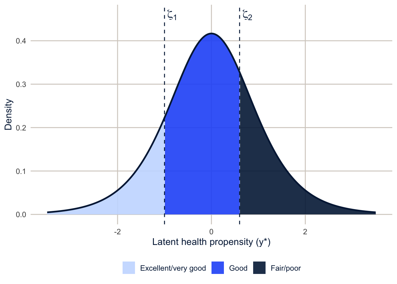
You don’t need to write code like this yourself; it draws the picture. dlogis() gives the height of the logistic distribution, cut() labels each point by the interval it falls in, geom_area() shades the areas, and annotate() adds the \(\zeta\) labels.
The proportional odds model is a set of \(J-1\) binary logits for the cumulative probabilities:
\[ \text{logit}\, P(y_i \le j) = \zeta_j - \mathbf{x}_i'\boldsymbol\beta, \qquad j = 1, \dots, J-1 \]
With our three categories, ordered from best (excellent or very good) to worst (fair or poor), \(J = 3\) and the model is two equations:
\[ \begin{aligned} \text{logit}\, P(\text{excellent or very good}) &= \zeta_1 - \mathbf{x}_i'\boldsymbol\beta \\ \text{logit}\, P(\text{good or better}) &= \zeta_2 - \mathbf{x}_i'\boldsymbol\beta \end{aligned} \]
So each equation models the probability of being at or below a cut point, which here means in that category or a better one. Because of the minus sign, a positive \(\beta\) lowers both of those probabilities, which pushes people toward the worse categories. If the categories were ordered from worst to best instead, every sign would flip. The model would be the same, but you’d read it the other way. So before you interpret any coefficient, check which end of the scale is “high,” and don’t rely on the sign alone; the predicted probabilities below make the direction unambiguous.
Each split of the outcome gets its own intercept \(\zeta_j\), but the coefficients \(\boldsymbol\beta\) are the same for every split. That is the proportional odds (or parallel lines) assumption. It says that education, say, shifts the odds of being in a worse category by the same factor whether we’re comparing fair or poor to everything better, or good or worse to excellent or very good. With three categories there are only two splits, so the assumption is easy to look at directly.
On the log-odds scale, the assumption means the model is a set of parallel lines, one for each split, with different intercepts and the same slope: a shared slope across the cumulative comparisons. The left panel of Figure 5.2 shows that. The right panel shows what a violation looks like: \(x\) has a steeper slope for one split than for the other, so its effect depends on which comparison you make.
tibble(x = seq(0, 6, by = 0.1)) |>
  cross_join(tibble(split = c("P(y > 1)", "P(y > 2)"), intercept = c(1, -1.5),
                    slope_violated = c(0.2, 0.7))) |>
  mutate(`Proportional odds holds` = intercept + 0.4 * x,
         `Proportional odds violated` = intercept + slope_violated * x) |>
  pivot_longer(starts_with("Proportional"), names_to = "panel", values_to = "log_odds") |>
  ggplot(aes(x = x, y = log_odds, colour = split, linetype = split)) +
  geom_line(linewidth = 1.2) +
  facet_wrap(~panel) +
  scale_colour_utsa(palette = "primary") +
  labs(x = "x", y = "Cumulative log odds", colour = NULL, linetype = NULL)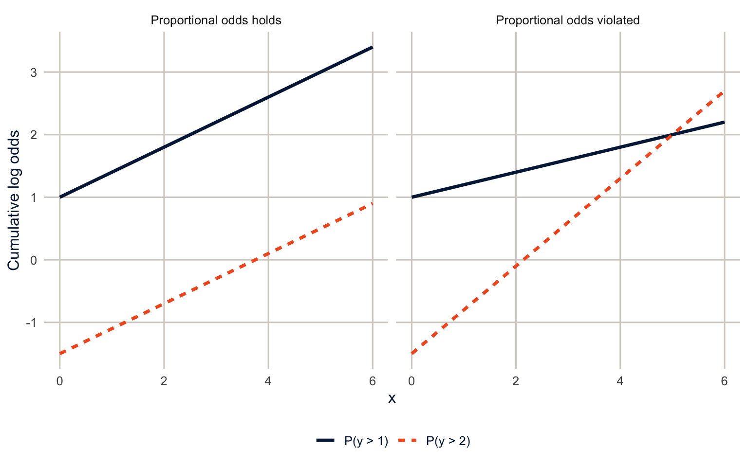
The model is attractive because each \(\beta\) has a single, consistent interpretation. The assumption can be a weak one in practice, though, because some covariates may affect certain transitions more than others, and I’ll show how to check it below.
fit_po <- svyolr(genhlth3 ~ race_eth + educ + agec + female, design = des)
summary(fit_po)
#> Call:
#> svyolr(genhlth3 ~ race_eth + educ + agec + female, design = des)
#>
#> Coefficients:
#> Value Std. Error t value
#> race_ethNH Black 0.39706197 0.02573562 15.428501
#> race_ethNH Other 0.33245344 0.03842662 8.651645
#> race_ethNH Multiracial 0.38059454 0.05313220 7.163162
#> race_ethHispanic 0.44884497 0.02765628 16.229403
#> educHS graduate -0.69199477 0.04025400 -17.190708
#> educSome college -0.94511797 0.04074232 -23.197450
#> educCollege graduate -1.53977761 0.03922190 -39.258106
#> agec25-34 0.31274757 0.03581278 8.732849
#> agec35-44 0.40400581 0.03636483 11.109794
#> agec45-54 0.59404849 0.03738926 15.888211
#> agec55-64 0.76236943 0.03584879 21.266253
#> agec65+ 0.90399608 0.03361296 26.894272
#> female 0.08943837 0.01773361 5.043440
#>
#> Intercepts:
#> Value Std. Error t value
#> Excellent/very good|Good -0.3577 0.0495 -7.2330
#> Good|Fair/poor 1.3683 0.0496 27.5939
#> (6410 observations deleted due to missingness)svyolr() (“survey ordinal logistic regression”) fits the proportional odds model to the design. The outcome must be an ordered factor. In the summary(), the rows for the predictors are the \(\beta\)s, and the rows labeled with two category names separated by | are the cut points \(\zeta_j\).
With the minus sign in the model, positive coefficients mean higher (here, worse) categories. Hispanic respondents have 1.57 times the odds of being in a worse health category than non-Hispanic White respondents, at any split, and college graduates have 0.21 times the odds of people without a high school diploma. The two intercepts are the cut points.
Predicted probabilities
Odds ratios for cumulative splits are hard to explain to anyone, so I go straight to predicted probabilities. avg_predictions() gives the average predicted probability of each category for each level of education, holding the other variables at their observed values. by = "educ" asks for one set of averages per education group. The result has a group column for the outcome category, and for each education group the probabilities of the three categories add up to 1.
po_pred <- avg_predictions(fit_po, by = "educ", wts = "(weights)")
po_pred
#>
#> Group educ Estimate Std. Error z Pr(>|z|) S
#> Excellent/very good Less than HS 0.223 0.01095 20.4 <0.001 304.7
#> Excellent/very good HS graduate 0.404 0.01975 20.5 <0.001 307.2
#> Excellent/very good Some college 0.454 0.01992 22.8 <0.001 380.1
#> Excellent/very good College graduate 0.601 0.01989 30.2 <0.001 664.0
#> Good Less than HS 0.384 0.01065 36.0 <0.001 942.1
#> Good HS graduate 0.380 0.00937 40.6 <0.001 Inf
#> Good Some college 0.364 0.01062 34.3 <0.001 851.9
#> Good College graduate 0.291 0.01305 22.3 <0.001 363.3
#> Fair/poor Less than HS 0.393 0.01730 22.7 <0.001 377.1
#> Fair/poor HS graduate 0.215 0.01570 13.7 <0.001 140.0
#> Fair/poor Some college 0.182 0.01314 13.8 <0.001 142.3
#> Fair/poor College graduate 0.108 0.00860 12.6 <0.001 117.9
#> 2.5 % 97.5 %
#> 0.2019 0.245
#> 0.3657 0.443
#> 0.4152 0.493
#> 0.5621 0.640
#> 0.3628 0.405
#> 0.3617 0.398
#> 0.3431 0.385
#> 0.2653 0.317
#> 0.3590 0.427
#> 0.1847 0.246
#> 0.1561 0.208
#> 0.0912 0.125
#>
#> Type: probspo_pred |>
as_tibble() |>
mutate(group = factor(group, levels = levels(brfss$genhlth3))) |>
ggplot(aes(x = educ, y = estimate, fill = group)) +
geom_col(colour = "white") +
scale_fill_manual(values = utsa_pal("blues", interpolate = TRUE)(4)[2:4]) +
scale_y_continuous(labels = scales::label_percent()) +
labs(x = NULL, y = "Average predicted probability", fill = NULL)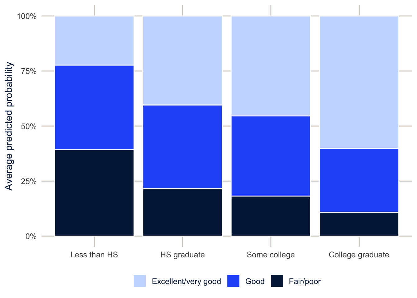
The model predicts that 39.3% of adults without a high school diploma report fair or poor health, compared with 10.8% of college graduates. The middle category behaves differently: the share in good health changes much less across education (38.4% versus 29.1%). That’s normal in ordinal models. The middle categories gain from one side and lose to the other, so their probabilities can move in either direction, and sometimes not at all.
TipReading the result: a right and a wrong interpretation
Right: “Comparing adults of the same race and ethnicity, age and sex, the model predicts that 39.3% of adults without a high school diploma report fair or poor health, against 10.8% of college graduates. The share reporting good health is similar in the two groups (38.4% and 29.1%).”
Wrong: “College graduates have a negative coefficient, so they’re less likely to be in every category below excellent or very good.” The coefficient says college graduates are less likely to be in a worse category at each cut point. It doesn’t say anything directly about the probability of a middle category, which can rise, fall or stay put. That’s why we report the predicted probabilities.
Note
I pass wts = "(weights)" so the averaging uses the survey weights. The standard errors come from the design-based variance of the coefficients through the delta method.
Checking the proportional odds assumption
A simple first look is to fit the binary logits for each split separately and compare the coefficients. This isn’t a formal test, but if the assumption holds, the two sets of coefficients should be close.
split1 <- svyglm(I(genhlth3 >= "Good") ~ race_eth + educ + agec + female,
                 design = des, family = quasibinomial())
split2 <- svyglm(I(genhlth3 == "Fair/poor") ~ race_eth + educ + agec + female,
                 design = des, family = quasibinomial())
I(genhlth3 >= "Good") makes a 0/1 outcome on the fly, as in week 1: TRUE (1) for good or fair/poor health. Comparing an ordered factor with >= uses the order of the levels.
list("Good or worse vs. better" = split1, "Fair/poor vs. better" = split2) |>
  map(\(m) broom::tidy(m, conf.int = TRUE)) |>
  list_rbind(names_to = "split") |>
  filter(term != "(Intercept)") |>
  mutate(term = str_remove_all(term, "race_eth|educ|agec"),
         term = fct_inorder(term)) |>
  ggplot(aes(x = estimate, y = fct_rev(term), colour = split, shape = split)) +
  geom_vline(xintercept = 0, colour = utsa_cols("smoke")) +
  geom_pointrange(aes(xmin = conf.low, xmax = conf.high),
                  position = position_dodge(width = 0.5)) +
  scale_colour_utsa(palette = "primary") +
  labs(x = "Logit coefficient", y = NULL, colour = NULL, shape = NULL)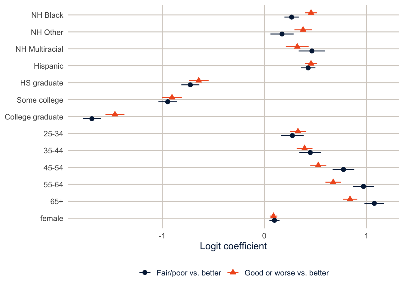
Most coefficients are close. Age is the exception: the older age groups have larger coefficients for the fair or poor split than for the good or worse split. In other words, getting older is associated with a bigger increase in the odds of fair or poor health than in the odds of merely good health.
Relaxing the assumption
svy_vglm() fits cumulative logit models in which some or all of the coefficients are allowed to differ across splits. The parallel argument controls which ones: parallel = TRUE is the proportional odds model, parallel = FALSE lets everything vary, and parallel = FALSE ~ agec lets only age vary. That last one is the partial proportional odds model.
fit_vpo <- svy_vglm(genhlth3 ~ race_eth + educ + agec + female, design = des,
                    family = cumulative(parallel = TRUE, reverse = TRUE))
fit_ppo <- svy_vglm(genhlth3 ~ race_eth + educ + agec + female, design = des,
                    family = cumulative(parallel = FALSE ~ agec, reverse = TRUE))
summary(fit_ppo)
#> svy_vglm.survey.design(genhlth3 ~ race_eth + educ + agec + female,
#> design = des, family = cumulative(parallel = FALSE ~ agec,
#> reverse = TRUE))
#> Stratified Independent Sampling design (with replacement)
#> svydesign(ids = ~1, strata = ~ststr, weights = ~mmsawt, data = brfss)
#> Coef SE z p
#> (Intercept):1 0.380494 0.050327 7.5604 4.019e-14
#> (Intercept):2 -1.462412 0.057373 -25.4897 < 2.2e-16
#> race_ethNH Black 0.392659 0.025979 15.1143 < 2.2e-16
#> race_ethNH Other 0.329108 0.039105 8.4160 < 2.2e-16
#> race_ethNH Multiracial 0.378044 0.052229 7.2383 4.544e-13
#> race_ethHispanic 0.448803 0.027546 16.2930 < 2.2e-16
#> educHS graduate -0.690490 0.040034 -17.2476 < 2.2e-16
#> educSome college -0.942399 0.040429 -23.3101 < 2.2e-16
#> educCollege graduate -1.534704 0.038969 -39.3824 < 2.2e-16
#> agec25-34:1 0.333797 0.038917 8.5771 < 2.2e-16
#> agec25-34:2 0.254770 0.055389 4.5996 4.233e-06
#> agec35-44:1 0.404636 0.039483 10.2483 < 2.2e-16
#> agec35-44:2 0.421310 0.053923 7.8132 5.577e-15
#> agec45-54:1 0.545899 0.039984 13.6530 < 2.2e-16
#> agec45-54:2 0.735997 0.053068 13.8690 < 2.2e-16
#> agec55-64:1 0.690467 0.038861 17.7676 < 2.2e-16
#> agec55-64:2 0.938734 0.050549 18.5709 < 2.2e-16
#> agec65+:1 0.841956 0.036064 23.3459 < 2.2e-16
#> agec65+:2 1.055013 0.047935 22.0091 < 2.2e-16
#> female 0.090197 0.017744 5.0832 3.711e-07svy_vglm() takes a formula and a design like svyglm(), and the family says which model. cumulative() is the family of cumulative logit models; parallel sets which coefficients are shared across splits, and reverse = TRUE flips the direction of the cumulative probabilities. There’s a lot in the summary. You don’t need to read every line; we’ll use predicted probabilities to compare the models.
VGAM writes the model as \(\text{logit}\, P(y \ge j+1) = \alpha_j + \mathbf{x}'\boldsymbol\beta\) when reverse = TRUE, so the slopes have the same sign as in svyolr() and the intercepts have the opposite sign. The age coefficients now come in pairs, with :1 for the first split and :2 for the second.
To test whether age needs separate coefficients, I use a design-based Wald test that the pairs are equal. The idea is simple: for each age group, take the difference between its two coefficients (one per split), and ask whether all those differences could be zero, given their standard errors. The code below does that with matrix algebra. It’s optional to follow line by line; the result (the p-value) is what matters.
b <- fit_ppo$coef
V <- fit_ppo$var
age_terms <- unique(str_remove(grep("^agec", names(b), value = TRUE), ":[12]$"))

L <- matrix(0, nrow = length(age_terms), ncol = length(b),
            dimnames = list(age_terms, names(b)))
for (a in age_terms) {
  L[a, paste0(a, ":1")] <- 1
  L[a, paste0(a, ":2")] <- -1
}

diffs <- L %*% b
wald <- drop(t(diffs) %*% solve(L %*% V %*% t(L)) %*% diffs)
c(chisq = wald, df = nrow(L),
  p = pchisq(wald, df = nrow(L), lower.tail = FALSE))
#> chisq df p
#> 9.287146e+01 5.000000e+00 1.674219e-18
NoteCode explanation: the Wald test by hand (optional)
b and V are the coefficients and their design-based variance-covariance matrix, stored in the fit. The grep() and str_remove() line lists the age terms. L is a contrast matrix with one row per age group, holding a 1 for that age group’s first-split coefficient and a \(-1\) for its second-split coefficient, so L %*% b (%*% is matrix multiplication) gives the differences. The Wald statistic is \(d'(LVL')^{-1}d\), where \(d\) is the vector of differences; solve() takes the matrix inverse and t() the transpose. Under the hypothesis that every difference is zero, it has a \(\chi^2\) distribution with one degree of freedom per difference, and pchisq(..., lower.tail = FALSE) gives the p-value.
The test rejects equality, so the partial proportional odds model is the better description of these data. Is the difference big enough to matter? In a sample of this size, almost any departure from proportional odds will be “significant,” so look at the coefficients too. The race, education and sex effects barely move between the two models, which tells you the substantive conclusions about them don’t depend on the assumption.
Tip
You’ll see the Brant test recommended for checking proportional odds. It’s a fine test for simple random samples, but it doesn’t account for survey design, and the Wald test above does. You’ll also see people compare pseudo-AIC values computed from survey models. Weighted pseudo-likelihoods aren’t true likelihoods, so I don’t trust AIC comparisons built on them.
Unordered outcomes
The multinomial logit model
The natural distribution for an outcome with \(J\) unordered categories is the multivariate extension of the binomial, the multinomial. If \(\pi_1, \pi_2, \dots, \pi_J\) are the probabilities of the categories (with \(\sum_j \pi_j = 1\)), and we observe \(y_1\) outcomes in the first category, \(y_2\) in the second and so on, with \(\sum_j y_j = n\), then
\[ f(\mathbf{y} \mid n) = \frac{n!}{y_1!\, y_2! \cdots y_J!}\, \pi_1^{y_1} \pi_2^{y_2} \cdots \pi_J^{y_J} \]
With \(J = 2\) this is just the binomial. For an individual respondent, \(n = 1\), and one of the \(y_j\) is 1 and the rest are 0.
When the categories have no natural order, we pick one as the reference and model the log odds of each other category relative to it. With \(J\) categories there are \(J-1\) equations, each with its own set of coefficients:
\[ \log \frac{P(y_i = j)}{P(y_i = \text{ref})} = \mathbf{x}_i'\boldsymbol\beta_j, \qquad j \ne \text{ref} \]
and the probabilities come from putting them back together:
\[ P(y_i = j) = \frac{\exp(\mathbf{x}_i'\boldsymbol\beta_j)}{\sum_{k} \exp(\mathbf{x}_i'\boldsymbol\beta_k)}, \qquad \boldsymbol\beta_{\text{ref}} = \mathbf{0} \]
That’s a lot of coefficients. With three categories every predictor gets two of them, and the exponentiated coefficients (relative risk ratios) compare each category to the reference, not to “everything else.” Predicted probabilities are even more important here than in the ordinal model.
The multinomial logit also assumes the independence of irrelevant alternatives (IIA): the odds of choosing A over B don’t depend on whether C is available. The classic example of where it fails: suppose commuters choose between driving and a red bus, half and half. Add a blue bus that’s identical to the red one. Realistically, the bus riders split between the two buses and drivers keep driving, so driving stays at half. But IIA forces the odds of driving versus the red bus to stay the same, so the model would put driving at a third. The assumption is questionable whenever two categories are close substitutes. Formal tests for IIA perform poorly, so the practical advice is to think about whether your categories are distinct alternatives that people actually choose among, and to avoid near-duplicate categories (Long and Freese 2014).
The reference outcome matters for reading the coefficients but not for the predictions. Every equation compares one category with the reference, so changing the reference changes every coefficient (they now compare with a different category), but the predicted probabilities of each category stay exactly the same. Exercise 4 asks you to check this.
The data: contraceptive use and intentions
I’ll use the DHS model dataset again, now for currently married or cohabiting women. DHS asks women who aren’t using contraception whether they intend to use it later, which gives three categories: using a method, not using but intending to, and not using with no intention to.
dhs <- get_dhs_model() |>
  filter(v502 == 1) |>
  mutate(fp = factor(case_when(v364 %in% 1:2 ~ "Using",
                               v364 == 3 ~ "Intends to use",
                               v364 == 4 ~ "No intention"),
                     levels = c("Using", "Intends to use", "No intention")),
         age = v012,
         children = v218,
         educ = factor(v106, 0:3, c("None", "Primary", "Secondary", "Higher")),
         wealth = factor(v190, 1:5, c("Poorest", "Poorer", "Middle", "Richer", "Richest")),
         rural = factor(v025, 1:2, c("Urban", "Rural")),
         wt = v005 / 1e6)

table(dhs$educ, dhs$fp)
#>
#> Using Intends to use No intention
#> None 552 1492 1821
#> Primary 126 326 223
#> Secondary 178 367 191
#> Higher 37 35 32The DHS design has clusters (v021), strata (v022), and a weight (v005) with six implied decimal places. Cluster numbers repeat across strata, so nest = TRUE.
dhs_des <- svydesign(ids = ~v021, strata = ~v022, weights = ~wt,
                     data = dhs, nest = TRUE)
svymean(~fp, dhs_des)
#> mean SE
#> fpUsing 0.17539 0.0092
#> fpIntends to use 0.40244 0.0120
#> fpNo intention 0.42217 0.0146v364 is the DHS contraceptive use and intention variable: codes 1 and 2 are using a method, 3 is not using but intends to, and 4 is not using with no intention. filter(v502 == 1) keeps women who are currently married or living with a partner.
Fitting the model
fit_mn <- svy_vglm(fp ~ age + I(age^2) + children + educ + wealth + rural,
                   design = dhs_des,
                   family = multinomial(refLevel = "Using"))
summary(fit_mn)
#> svy_vglm.survey.design(fp ~ age + I(age^2) + children + educ +
#> wealth + rural, design = dhs_des, family = multinomial(refLevel = "Using"))
#> Stratified 1 - level Cluster Sampling design (with replacement)
#> With (217) clusters.
#> svydesign(ids = ~v021, strata = ~v022, weights = ~wt, data = dhs,
#> nest = TRUE)
#> Coef SE z p
#> (Intercept):1 4.16005594 0.83742642 4.9677 6.776e-07
#> (Intercept):2 5.75696831 0.82464201 6.9812 2.927e-12
#> age:1 -0.16637316 0.05353515 -3.1077 0.0018853
#> age:2 -0.31261649 0.04876549 -6.4106 1.449e-10
#> I(age^2):1 0.00197825 0.00076557 2.5840 0.0097660
#> I(age^2):2 0.00542811 0.00070425 7.7076 1.282e-14
#> children:1 -0.11482843 0.03169620 -3.6228 0.0002915
#> children:2 -0.28354062 0.03263935 -8.6871 < 2.2e-16
#> educPrimary:1 -0.10879839 0.14510697 -0.7498 0.4533869
#> educPrimary:2 -0.49198840 0.16162089 -3.0441 0.0023339
#> educSecondary:1 -0.31340581 0.18143318 -1.7274 0.0840977
#> educSecondary:2 -0.95435598 0.21676772 -4.4027 1.069e-05
#> educHigher:1 -0.90189534 0.27620173 -3.2654 0.0010933
#> educHigher:2 -1.75201979 0.44976266 -3.8954 9.802e-05
#> wealthPoorer:1 0.02863509 0.15059989 0.1901 0.8491993
#> wealthPoorer:2 -0.03069719 0.14734460 -0.2083 0.8349666
#> wealthMiddle:1 0.05917347 0.16179329 0.3657 0.7145628
#> wealthMiddle:2 -0.05046086 0.16054973 -0.3143 0.7532928
#> wealthRicher:1 -0.11387436 0.17081414 -0.6667 0.5049916
#> wealthRicher:2 -0.45115850 0.20114309 -2.2430 0.0248986
#> wealthRichest:1 -0.13174172 0.22141239 -0.5950 0.5518394
#> wealthRichest:2 -0.07560169 0.26970612 -0.2803 0.7792386
#> ruralRural:1 0.56907897 0.14304058 3.9784 6.937e-05
#> ruralRural:2 0.77513298 0.18115153 4.2789 1.878e-05multinomial(refLevel = "Using") is the multinomial logit family, with “Using” as the reference outcome. The summary is long: two coefficients for every predictor. Skim it for the structure, then move on to the predicted probabilities, which are what you’d report.
Each coefficient ending in :1 belongs to the equation for “intends to use” versus “using,” and each ending in :2 belongs to “no intention” versus “using.” Rural women have 2.17 times the relative risk of having no intention to use (rather than using) compared with urban women, holding the other variables constant. Secondary education is associated with lower relative risks of both non-use categories, and much more so for no intention (0.39) than for intending to use (0.73).
Predicted probabilities
svy_vglm() keeps the underlying vglm fit in $fit, and its predict() method returns the probability of each category. To get the average predicted probability for each level of education, I set every woman’s education to that level, predict, and take the weighted average. These are the same counterfactual averages that avg_predictions() computes, done by hand.
mn_pred <- levels(dhs$educ) |>
  set_names() |>
  map(\(e) {
    nd <- mutate(dhs, educ = factor(e, levels = levels(dhs$educ)))
    p <- predict(fit_mn$fit, newdata = nd, type = "response")
    tibble(outcome = colnames(p),
           probability = colSums(p * dhs$wt) / sum(dhs$wt))
  }) |>
  list_rbind(names_to = "educ") |>
  mutate(educ = factor(educ, levels = levels(dhs$educ)),
         outcome = factor(outcome, levels = levels(dhs$fp)))

mn_pred |>
  pivot_wider(names_from = outcome, values_from = probability) |>
knitr::kable(digits = 3)| educ | Using | Intends to use | No intention |
|---|---|---|---|
| None | 0.152 | 0.385 | 0.464 |
| Primary | 0.191 | 0.438 | 0.371 |
| Secondary | 0.241 | 0.454 | 0.305 |
| Higher | 0.372 | 0.403 | 0.225 |
NoteCode explanation: average predicted probabilities by hand
This is the map() pattern again, once per education level e:
mutate(dhs, educ = factor(e, levels = levels(dhs$educ)))makes a copy of the data in which every woman has educatione(keeping the same factor levels, so the model recognizes them).predict(fit_mn$fit, newdata = nd, type = "response")gives a matrix of predicted probabilities, one row per woman and one column per outcome category.type = "response"asks for probabilities rather than log-odds.colSums(p * dhs$wt) / sum(dhs$wt)is the weighted average of each column: multiply each woman’s probabilities by her weight, add up each column, and divide by the total weight.
mn_pred |>
  ggplot(aes(x = educ, y = probability, colour = outcome, group = outcome,
             shape = outcome)) +
  geom_line(linewidth = 1) +
  geom_point(size = 3) +
  scale_colour_utsa() +
  scale_y_continuous(labels = scales::label_percent(), limits = c(0, NA)) +
  labs(x = "Education", y = "Average predicted probability",
       colour = NULL, shape = NULL)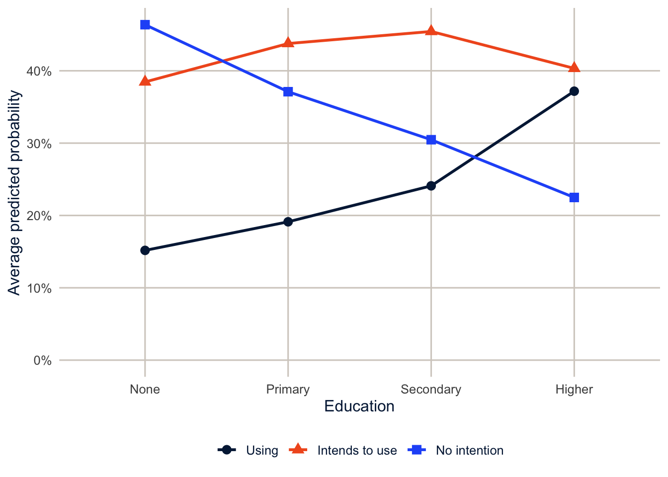
The picture is clearer than the table of coefficients. Moving from no education to higher education, the predicted probability of using a method rises from 15.2% to 37.2%, and the probability of having no intention to use falls from 46.4% to 22.5%. The intending-to-use category changes much less (it rises a little and then falls), because what it gains from “no intention” it loses to “using.” That’s the kind of pattern a binary model of use versus non-use would hide.
One caution: only 104 women in the sample have higher education, so the estimates for that group are much less precise than the others.
Warning
These predicted probabilities don’t come with standard errors. nnet::multinom() with marginaleffects will give you standard errors, but they treat the weights as if the data were a simple random sample, and with clustered DHS data they are much too small. For design-based intervals on predicted probabilities, repeat the calculation over replicate weights (exercise 3).
Back to self-rated health: ordered or not?
Nothing stops us from fitting a multinomial model to an ordered outcome. It just ignores the ordering, and it spends a lot more parameters doing so: two full sets of coefficients instead of one set plus two cut points. Comparing it with the ordinal models is a useful check on how much the proportional odds structure is costing us.
brfss_mn <- brfss |>
  mutate(genhlth_u = factor(genhlth3, ordered = FALSE))
des_mn <- svydesign(ids = ~1, strata = ~ststr, weights = ~mmsawt, data = brfss_mn)

fit_srh_mn <- svy_vglm(genhlth_u ~ race_eth + educ + agec + female, design = des_mn,
                       family = multinomial(refLevel = "Excellent/very good"))

round(exp(fit_srh_mn$coef[grep("^educ|^race_ethHispanic", names(fit_srh_mn$coef))]), 2)
#> race_ethHispanic:1 race_ethHispanic:2 educHS graduate:1
#> 1.47 1.84 0.68
#> educHS graduate:2 educSome college:1 educSome college:2
#> 0.39 0.54 0.28
#> educCollege graduate:1 educCollege graduate:2
#> 0.36 0.11factor(genhlth3, ordered = FALSE) turns the ordered factor into a plain one, so the multinomial model treats the categories as unordered. The last line exponentiates the coefficients whose names start with educ or race_ethHispanic (^ means “starts with” in a pattern).
Here the reference category is excellent or very good health, so every coefficient ending in :1 compares good health with excellent or very good, and every one ending in :2 compares fair or poor health with excellent or very good. College graduates have 0.36 times the relative risk of good (rather than excellent or very good) health compared with adults who didn’t finish high school, and 0.11 times the relative risk of fair or poor health. Education matters for both comparisons, and much more for the second. That’s the same thing the split logits showed us, seen from a different angle.
The way to compare the three models is through their predicted probabilities. I use the same set-everyone’s-education-and-average approach as for the DHS model, on the respondents used to fit the models.
srh_cc <- brfss_mn |>
  filter(complete.cases(genhlth_u, race_eth, educ, agec, female))

avg_probs <- function(fit, data) {
  levels(data$educ) |>
    set_names() |>
    map(\(e) {
      nd <- mutate(data, educ = factor(e, levels = levels(data$educ)))
      p <- predict(fit, newdata = nd, type = "response")
      tibble(outcome = colnames(p),
             probability = colSums(p * data$mmsawt) / sum(data$mmsawt))
    }) |>
    list_rbind(names_to = "educ")
}

srh_pred <- list("Proportional odds" = fit_vpo$fit,
                 "Partial proportional odds" = fit_ppo$fit,
                 "Multinomial" = fit_srh_mn$fit) |>
  map(\(f) avg_probs(f, srh_cc)) |>
  list_rbind(names_to = "model") |>
  mutate(model = fct_inorder(model),
         educ = factor(educ, levels = levels(brfss$educ)),
         outcome = factor(outcome, levels = levels(brfss$genhlth3)))

srh_pred |>
  pivot_wider(names_from = model, values_from = probability) |>
  arrange(outcome, educ) |>
knitr::kable(digits = 3)| educ | outcome | Proportional odds | Partial proportional odds | Multinomial |
|---|---|---|---|---|
| Less than HS | Excellent/very good | 0.249 | 0.249 | 0.262 |
| HS graduate | Excellent/very good | 0.394 | 0.395 | 0.396 |
| Some college | Excellent/very good | 0.454 | 0.455 | 0.459 |
| College graduate | Excellent/very good | 0.598 | 0.598 | 0.594 |
| Less than HS | Good | 0.392 | 0.394 | 0.368 |
| HS graduate | Good | 0.384 | 0.384 | 0.381 |
| Some college | Good | 0.364 | 0.363 | 0.354 |
| College graduate | Good | 0.292 | 0.291 | 0.306 |
| Less than HS | Fair/poor | 0.360 | 0.357 | 0.370 |
| HS graduate | Fair/poor | 0.222 | 0.221 | 0.223 |
| Some college | Fair/poor | 0.182 | 0.182 | 0.188 |
| College graduate | Fair/poor | 0.110 | 0.110 | 0.100 |
avg_probs() wraps the by-hand calculation above in a function, so it can be run on each of the three models with map(). The averages use only the complete cases, the respondents the models were fit to.
The three models tell the same story. The two ordinal models are nearly identical, and the proportional odds and multinomial predictions never differ by more than 2.4 percentage points. With only three categories and a large sample, the proportional odds model is a good summary of the education gradient, even though we know from the Wald test that the assumption doesn’t hold exactly for age. So the choice among them comes down to what you want to say. The proportional odds model gives one coefficient per variable and is the easiest to explain. The partial proportional odds model relaxes the assumption only where the data say it needs relaxing. The multinomial is the most flexible, but it throws away the ordering and gives you twice as many coefficients to interpret.
Homework 5
Due: February 25, before class.
Which version to do. If you’re in DEM 7283, do the version with your own survey data. If you’re in DEM 5283, do either version, and say at the top of your homework which one you did. If your survey can’t support this week’s method, do the version with my data and say so.
Purpose. Match the model to the kind of outcome, check the assumption the model makes, and report the results as probabilities.
A satisfactory answer says what kind of outcome each one is and why; reports predicted probabilities for every category, checking that they add up to 1 for each group; and describes results as associations.
With your own survey data
Use the full survey design for every estimate unless a step says otherwise, and report each estimate with a standard error or confidence interval.
- Define an ordinal or multinomial outcome variable of your choosing, and explain how you recoded the original variable.
- Is your outcome ordered or unordered? Explain why in a sentence or two.
- If it’s ordered, why shouldn’t its categories be treated as equally spaced numbers?
- State a research question about the factors you believe will affect your outcome variable.
- Fit either an ordinal logistic regression (proportional odds model) or a multinomial logistic regression model to your outcome, using the survey design (
svyolr()orsvy_vglm()).- If you use an ordinal model, are the assumptions of the proportional odds model met?
- How did you evaluate the proportional odds assumption? Fit the model with
parallel = FALSEand use Wald tests to identify which variables violate it. - If a variable violates the assumption, fit a partial proportional odds model and say how your conclusions change.
- For the best-fitting model from the previous step:
- describe the results; and
- present a table showing odds ratios and confidence intervals for all model parameters.
- Report predicted probabilities for every category of your outcome for at least two groups that matter for your research question, and check that each group’s probabilities add up to 1.
With my data
What is provided. The BRFSS data with recode_mmsa() and the design des (the outcome genhlth3 is ordered from excellent or very good to fair or poor); the DHS design dhs_des and the multinomial model from this chapter, with “Using” as the reference outcome.
1. Explain in a sentence or two why genhlth3 is an ordinal outcome, and why its categories shouldn’t be treated as equally spaced numbers. Fit the proportional odds model for genhlth3 with income (income) added. Using avg_predictions(), report the predicted probability of every health category for adults in the lowest and the highest income groups, and check that each group’s probabilities add up to 1. Then describe the proportional odds assumption in your own words, and say what you would examine if it seemed unreasonable for income.
# YOUR CODE HERE2. Use the five-category version of self-rated health (genhlth, codes 1 to 5) as an ordered factor. Fit the proportional odds model and the model with parallel = FALSE for all variables. Which variables seem to violate proportional odds? Use the Wald test approach from this document.
# YOUR CODE HERE3. Convert the DHS design to a bootstrap replicate design with as.svrepdesign(dhs_des, type = "bootstrap", replicates = 100). Write a function that fits the multinomial model with a given set of weights and returns the average predicted probability of “Using” for women with no education and with secondary education. Run it over the replicate weights and report a standard error for each.
# YOUR CODE HEREA hint for exercise 3
VGAM::vglm() takes a weights argument, and vglm(..., weights = w) gives the same point estimates as svy_vglm() when w is the design weight. Loop over the columns of weights(rep_des, "analysis"), collect the two probabilities from each replicate, and pass the matrix of replicate estimates to svrVar() along with the design’s scale, rscales and the full-sample estimates.
4. Re-fit the multinomial model with “No intention” as the reference category. Show that the predicted probabilities don’t change, and explain in a sentence why the coefficients do.
# YOUR CODE HEREAdditional resources
- Long and Freese (2014) has the best practical chapters on ordinal and multinomial models, including how to test the proportional odds assumption and how to present the results.
- The
svyVGAMpackage page links to Thomas Lumley’s vignette on fittingVGAMmodels, including partial proportional odds models, to survey data. - The Model to Meaning book covers predicted probabilities for categorical outcomes, which is how I’d present these models in a paper.