Week 7: Decomposition

Introduction

Almost every interesting demographic finding starts as a difference between two groups. Texas has a higher death rate than California. Women earn less than men. Hispanic adults are more likely to be uninsured than non-Hispanic White adults. The first question anyone asks about a difference like that is why, and the first honest answer is usually “partly because the groups are made up of different kinds of people, and partly because the same kinds of people have different outcomes in the two groups.” Decomposition methods put numbers on those two parts.

This week covers the two workhorses. Kitagawa decomposition splits a difference in crude rates into a part due to the rates themselves and a part due to population composition, using aggregate data like the death counts from week 6. Oaxaca-Blinder decomposition does the same thing with microdata and a regression model, splitting a gap in means into a part explained by differences in characteristics and a part that is unexplained. I’ll finish with the extension to binary outcomes, where the regression is a logit and the arithmetic needs a little more care. Along the way you’ll use the survey weights and replicate weights from week 2, because a decomposition is just another estimate, and it needs a standard error.

NoteThis week at a glance

The question. Texas and California have nearly the same crude death rate, men earn more than women, and Hispanic adults are more likely to be uninsured. How much of each difference goes along with differences in who is in each group, and how much with differences in outcomes for the same kinds of people?

By the end of this week you should be able to

1. compute a Kitagawa decomposition by hand, and show that its two parts add up to the difference;
2. run an Oaxaca-Blinder decomposition with survey weights, report the gap and both components in the same units, and say which reference coefficients you used;
3. explain why the explained part isn’t a causal effect and the unexplained part isn’t a measure of discrimination.

Before you begin. You need crude and age-specific rates and the Texas and California data from week 6, linear regression, the IPUMS data and replicate weights from week 2, and predicted probabilities from week 3.

Required and optional. Splitting the explained part of a binary-outcome decomposition into individual variables is an extension, and so is the by-hand matrix version of Oaxaca-Blinder.

When it’s due. Homework 7 is due before class on March 18, the first class after spring break.

Setup

We need the Texas and California mortality data from week 6, the IPUMS ACS extract for Texas from week 2, and the BRFSS. The oaxaca package does the linear decomposition in one line (Hlavac 2022), but it doesn’t know about survey weights. So for the regression decompositions, we’ll use svy_oaxaca(), a function I wrote for this course. It’s in the course’s R/ folder, next to get_mmsa(). It takes a survey design object, the same kind you’ve been passing to svyglm() since week 2. Because it comes from a file you source() and not from a package, ?svy_oaxaca won’t find its help page. Run svy_oaxaca_help() instead, which opens the same kind of page in the Viewer.

library(tidyverse)
library(here)
library(survey)
library(srvyr)
library(ipumsr)
library(oaxaca)
library(sparkscolors)  # pak::pak("coreysparks/sparkscolors"), UTSA colors

source(here("R", "get_mmsa.R"))
source(here("R", "recode_mmsa.R"))
source(here("R", "svy_oaxaca.R"))

Why decompose?

Demographers have been decomposing differences for as long as there have been rates to compare. The logic goes back to standardization, which you saw in week 6: a crude death rate mixes the risk of dying at each age with the number of people at each age, and if two populations have different age structures, their crude rates can mislead you. Standardization answers one counterfactual question (“what would Texas’s death rate be with California’s age structure?”). Decomposition answers a slightly different one: of the actual difference between the two crude rates, how much comes from the rates and how much from the age structure?

Every decomposition in this document has the same shape:

\[\text{difference} = \text{part due to composition} + \text{part due to rates (or coefficients)}\]

Different fields use different names for the two parts. Demographers say composition and rate effects. Economists, who developed the regression version, say explained (or endowments) and unexplained (or coefficients). They’re the same idea.

Before we start, one warning that I’ll repeat at the end. A decomposition is accounting, not causal inference. It divides an observed difference into components under a chosen accounting rule. It doesn’t tell you what would happen if a policy changed someone’s education or moved them to California, and its unexplained component isn’t a direct estimate of discrimination. We’ll come back to that distinction in week 14.

Part 1: Kitagawa decomposition

The idea

A crude death rate is a weighted average of age-specific death rates, where the weights are the shares of the population in each age group. If \(c_i\) is the share of the population in age group \(i\) and \(m_i\) is the death rate in that group, then

\[CDR = \sum_i c_i m_i\]

Before the formula, here is the whole idea with two made-up populations and just two age groups, young and old. Rates are deaths per 1,000.

	Population A: share	Population A: rate	Population B: share	Population B: rate
Young	0.8	2	0.6	2
Old	0.2	50	0.4	40
Crude rate		\(0.8 \times 2 + 0.2 \times 50 = 11.6\)		\(0.6 \times 2 + 0.4 \times 40 = 17.2\)

Population A’s old people die at a higher rate (50 against 40), and young people die at the same rate in both. Yet A’s crude rate is lower, by \(11.6 - 17.2 = -5.6\), because A has far fewer old people. A crude difference can reflect differences in the rates, differences in composition, or both, pulling in opposite directions.

For two populations \(A\) and \(B\), Kitagawa (1955) showed that the difference in crude rates can be split exactly into two parts:

\[CDR_A - CDR_B = \underbrace{\sum_i \frac{c_{iA} + c_{iB}}{2}(m_{iA} - m_{iB})}_{\text{rate effect}} + \underbrace{\sum_i \frac{m_{iA} + m_{iB}}{2}(c_{iA} - c_{iB})}_{\text{composition effect}}\]

The rate effect asks how different the death rates are, weighting each age by its average share of the two populations. The composition effect asks how different the age structures are, weighting each age by its average death rate. Using the averages of the two populations, rather than one or the other, is what makes the two parts add up exactly to the total, with nothing left over. You can check the algebra yourself: multiply out the two sums and the cross terms cancel. Preston et al. (2001) walk through it, and Das Gupta (1993) extends it to rates with more than two factors (age, sex and race at once, for example).

Here’s every term for the small example. The rate effect weights each difference in rates by the average share of the two populations in that age group:

• young: \(\frac{0.8 + 0.6}{2} \times (2 - 2) = 0.7 \times 0 = 0\)
• old: \(\frac{0.2 + 0.4}{2} \times (50 - 40) = 0.3 \times 10 = 3.0\)
• total rate effect: \(0 + 3.0 = 3.0\)

The composition effect weights each difference in shares by the average rate in that age group:

• young: \(\frac{2 + 2}{2} \times (0.8 - 0.6) = 2 \times 0.2 = 0.4\)
• old: \(\frac{50 + 40}{2} \times (0.2 - 0.4) = 45 \times (-0.2) = -9.0\)
• total composition effect: \(0.4 - 9.0 = -8.6\)

And the two parts add up to the difference exactly: \(3.0 + (-8.6) = -5.6\). Population A’s higher old-age death rate would make its crude rate 3 points higher, and its younger age structure makes it 8.6 points lower. Keep this example in mind, because Texas and California turn out to look a lot like it.

Texas and California

Here are the 2016 deaths and populations by age from week 6.

age_levels <- c("< 1 year", "1-4 years", "5-9 years", "10-14 years", "15-19 years",
                "20-24 years", "25-34 years", "35-44 years", "45-54 years",
                "55-64 years", "65-74 years", "75-84 years", "85+ years")

txca <- read_tsv(here("data", "CMF_TX_CA_age.txt"), na = c("", "Not Applicable", "Suppressed"),
                 show_col_types = FALSE) |>
  rename(state = State, age = `Age Group`, deaths = Deaths, population = Population) |>
  filter(age != "Not Stated") |>
  mutate(age = factor(age, levels = age_levels),
         deaths = as.numeric(deaths), population = as.numeric(population)) |>
  select(state, age, deaths, population)

To do the decomposition, we need the age shares \(c_i\) and the rates \(m_i\) for each state, side by side in one row per age group.

kit <- txca |>
  group_by(state) |>
  mutate(c = population / sum(population),   # share of the population in each age group
         m = 1e5 * deaths / population) |>    # deaths per 100,000
  ungroup() |>
  select(state, age, c, m) |>
  pivot_wider(names_from = state, values_from = c(c, m)) |>
  mutate(rate_effect = (c_Texas + c_California) / 2 * (m_Texas - m_California),
         comp_effect = (m_Texas + m_California) / 2 * (c_Texas - c_California))

kit_total <- kit |>
  summarise(cdr_texas = sum(c_Texas * m_Texas),
            cdr_california = sum(c_California * m_California),
            difference = cdr_texas - cdr_california,
            rate_effect = sum(rate_effect),
            comp_effect = sum(comp_effect))

knitr::kable(kit_total, digits = 1)

cdr_texas	cdr_california	difference	rate_effect	comp_effect
689	668.1	20.9	116.1	-95.2

1e5 is R’s way of writing \(1 \times 10^5\), or 100,000, so m is deaths per 100,000.

NoteCode explanation: pivot_wider() with two value columns

The data start out “long,” with one row for each state and age group (26 rows). The formula needs Texas and California values next to each other, so we want them “wide,” with one row per age group (13 rows).

1. names_from = state says the new columns should be named after the values of state.
2. values_from = c(c, m) says to spread out two columns at once, the shares and the rates. When there’s more than one, pivot_wider() names the new columns by gluing the variable name to the state name with an underscore: c_Texas, c_California, m_Texas and m_California.
3. After that, each line of the Kitagawa formula is one mutate(), and each sum is one summarise().

pivot_longer() goes the other way, and you’ll use it below to get the data back into long form for plotting.

The crude death rate in Texas was 689.0 per 100,000, and in California 668.1, a difference of only 20.9. Looked at that way, the two states are nearly the same. The decomposition says otherwise. Texas’s higher age-specific death rates would have made its crude rate 116.1 points higher, but its younger population pulled it back down by 95.2. Two big effects in opposite directions add up to a small difference. That’s the same story as the age-standardized rate ratio of about 1.19 in week 6, but now it’s in the units of the crude rate, and it adds up.

The age-specific contributions show where each effect comes from.

kit |>
  select(age, `Rate effect` = rate_effect, `Composition effect` = comp_effect) |>
  pivot_longer(-age, names_to = "component", values_to = "contribution") |>
  ggplot(aes(x = age, y = contribution, fill = component)) +
  geom_col(position = "dodge") +
  geom_hline(yintercept = 0, colour = utsa_cols("midnight")) +
  scale_fill_utsa(palette = "primary") +
  labs(x = "Age group", y = "Contribution (deaths per 100,000)", fill = NULL) +
  theme(axis.text.x = element_text(angle = 45, hjust = 1))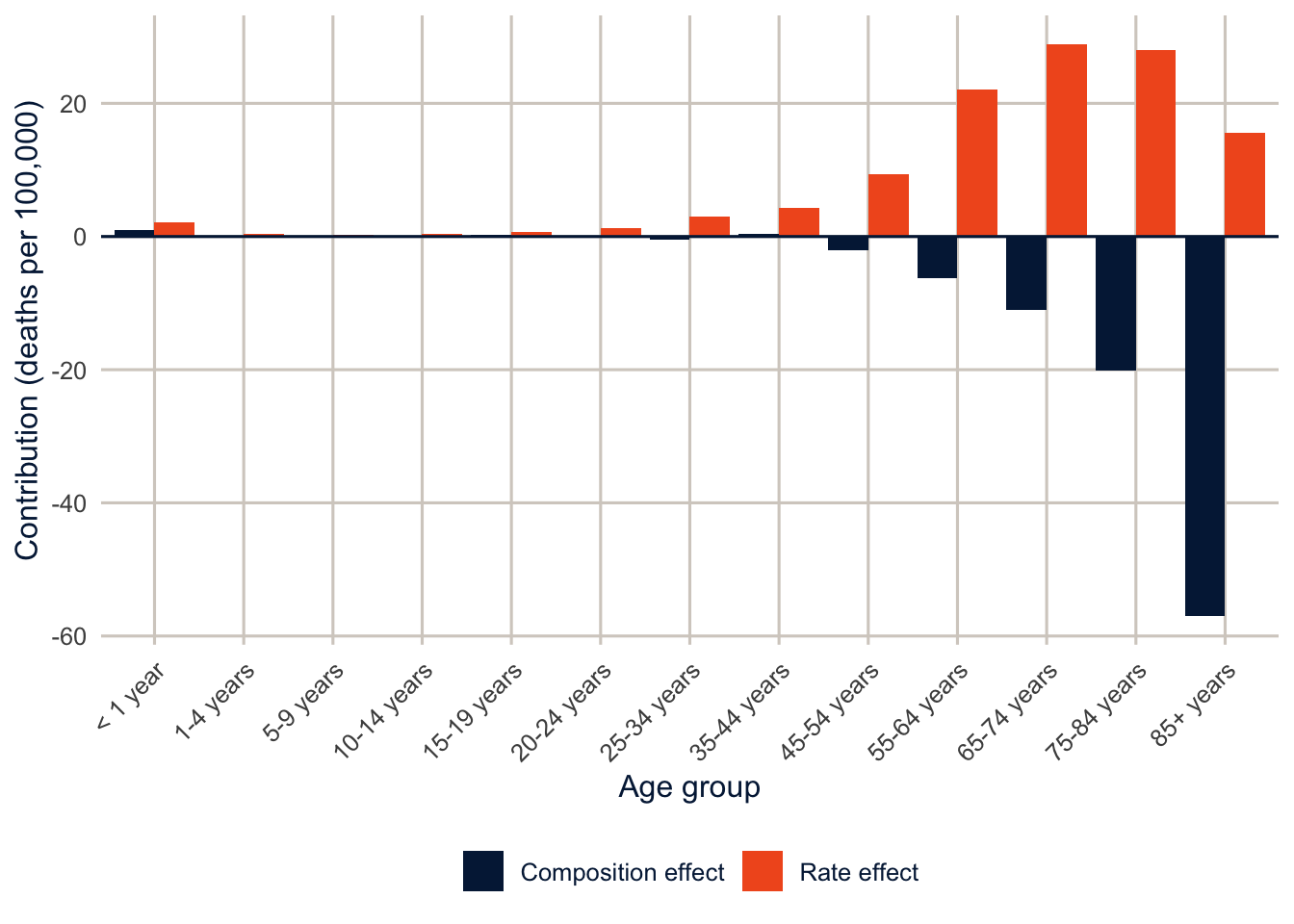

Figure 7.1: Contributions of each age group to the difference in crude death rates between Texas and California, 2016, deaths per 100,000.

The rate effect is positive at every age, so Texans die at higher rates than Californians across the whole life course, and the biggest contributions are from 55 to 84, where both the rate differences and the population shares are large. The composition effect is almost all at the oldest ages: California has a larger share of people over 85, and since that’s where the death rate is highest, that alone is worth 57.0 deaths per 100,000.

Tip

Two practical points. First, the age groups matter. Wide open-ended groups like 85+ hide age differences within the group, and those leak into the rate effect. Second, the same machinery works for any rate that’s a weighted average of group-specific rates: a total fertility rate across marital statuses, a poverty rate across family types, an employment rate across education groups. If you can write it as \(\sum c_i m_i\), you can decompose it.

Part 2: Oaxaca-Blinder decomposition

From rates to regressions

Kitagawa works with a handful of categories. With microdata, we usually want to account for many characteristics at once, some continuous, and that’s where a regression comes in. The goal is the same: we start from the observed gap between two groups, and we split it into a part that goes with differences in characteristics (composition) and a part that goes with differences in how characteristics relate to the outcome (rates). What changes is the accounting tool: instead of age-specific rates and shares, we use regression coefficients and group means. Oaxaca (1973) and Blinder (1973) independently proposed the same idea, in the same year, for the same question: how much of the gap in wages between groups is due to differences in productive characteristics, and how much is due to the groups being paid differently for the same characteristics?

Fit the same linear regression separately to two groups, \(A\) and \(B\):

\[y_{iA} = X_{iA}\beta_A + \varepsilon_{iA} \qquad y_{iB} = X_{iB}\beta_B + \varepsilon_{iB}\]

Because a linear regression with an intercept goes through the means, the mean outcome in each group is its mean characteristics times its coefficients, \(\bar y_A = \bar X_A \beta_A\). So the gap is

\[\bar y_A - \bar y_B = \bar X_A \beta_A - \bar X_B \beta_B\]

Now add and subtract a set of reference coefficients \(\beta^*\) and rearrange:

\[\bar y_A - \bar y_B = \underbrace{(\bar X_A - \bar X_B)\beta^*}_{\text{explained}} + \underbrace{\bar X_A(\beta_A - \beta^*) + \bar X_B(\beta^* - \beta_B)}_{\text{unexplained}}\]

The explained part is how much the gap would be if both groups were paid according to the same coefficients, so the only thing that differs is their characteristics. “Explained” is a technical word here, and it means much less than it sounds like: the part of the gap attributed to the measured characteristics in this model, using this choice of reference coefficients. It doesn’t mean causally explained. The unexplained part is everything else: differences in the coefficients, including the intercepts. It’s the same structure as Kitagawa, with \(\bar X\) playing the part of composition and \(\beta\) the part of the rates.

Choosing the reference coefficients

The decomposition is exact for any \(\beta^*\), but the split between explained and unexplained depends on which one you choose. The reason is easy to see in the formula. The explained part is the difference in characteristics times \(\beta^*\). If one group’s coefficients put a big value on education and the other’s a small one, the same difference in education is “worth” more under the first set. The observed gap doesn’t change at all; only the way it’s divided up does. This is the index number problem, and it’s the same reason Kitagawa used the average of the two populations. There are four common choices:

1. \(\beta^* = \beta_A\), the coefficients of the advantaged group, as in Oaxaca (1973). It treats group \(A\)’s wage structure as the “fair” one.
2. \(\beta^* = \beta_B\), the coefficients of the disadvantaged group.
3. The coefficients from a pooled regression on both groups (Neumark 1988).
4. The coefficients from a pooled regression that also includes a group indicator (Jann 2008; Fortin et al. 2011). Without the indicator, the pooled coefficients absorb some of the group difference, and part of the unexplained gap gets mislabeled as explained.

I’ll use the fourth as the main specification and show how much the others move things. There’s no right answer here, so you should always say which one you used.

The gender gap in wages in Texas

I’ll use the IPUMS extract of the 2024 ACS for Texas from week 2, and decompose the gap in log annual wages between men and women who were employed and between 25 and 64. Log wages are the convention, because the coefficients become approximate percent differences and the gap in mean log wages is (roughly) a percent gap.

ddi <- read_ipums_ddi(here("data", "usa_00014.xml"))
ipums <- read_ipums_micro(ddi, data_file = here("data", "usa_00014_tx.dat.gz"),
                          verbose = FALSE)

wages <- ipums |>
  filter(EMPSTAT == 1, between(AGE, 25, 64),
         INCWAGE > 0, INCWAGE < 999998) |>      # 999998 and 999999 are missing and N/A
  mutate(lnwage = log(INCWAGE),
         female = as.numeric(SEX == 2),
         educ = cut(EDUC, breaks = c(-1, 5, 6, 8, 10, 11),
                    labels = c("Less than HS", "HS graduate", "Some college",
                               "Bachelor's", "Graduate")),
         race_eth = case_when(HISPAN %in% 1:4 ~ "Hispanic",
                              RACE == 1 ~ "NH White",
                              RACE == 2 ~ "NH Black",
                              RACE %in% 4:6 ~ "NH Asian",
                              .default = "NH Other"),
         race_eth = fct_relevel(factor(race_eth), "NH White"),
         # first two digits of the SOC code = the 23 major occupation groups
         occ = factor(substr(OCCSOC, 1, 2)))

wages |>
  group_by(female) |>
  summarise(n = n(),
            mean_lnwage = weighted.mean(lnwage, PERWT),
            geometric_mean_wage = exp(mean_lnwage),
            bachelors_plus = weighted.mean(educ %in% c("Bachelor's", "Graduate"), PERWT),
            mean_age = weighted.mean(AGE, PERWT)) |>
  knitr::kable(digits = 3, format.args = list(big.mark = ","))

female	n	mean_lnwage	geometric_mean_wage	bachelors_plus	mean_age
0	52,968	10.991	59,338.40	0.381	42.381
1	47,887	10.622	41,009.58	0.450	42.425

Warning

My extract doesn’t have hours or weeks worked, so these are annual wages, and part of any gap between men and women in annual wages is a gap in how much they work. A real analysis would add usual hours (UHRSWORK) and weeks worked (WKSWORK2) to the extract, and either model hourly wages or restrict to full-time, full-year workers. Exercise 2 asks you to think about what that does to the decomposition.

In the recode, cut(EDUC, breaks = c(-1, 5, 6, 8, 10, 11), labels = ...) groups the IPUMS education codes into five categories (each category runs from just above one break to the next). case_when() with .default = "NH Other" gives everyone not matched by an earlier rule the last category, fct_relevel(..., "NH White") makes non-Hispanic White the first (reference) level, and substr(OCCSOC, 1, 2) keeps the first two characters of the occupation code.

Women in this sample are more likely than men to have a bachelor’s degree, and the two groups have the same average age. So education and age won’t explain the gap, and if anything, education will work against it.

The decomposition with svy_oaxaca()

First, the replicate design. This is the same as_survey_rep() call as in week 2, with the Census Bureau’s 80 replicate weights and its variance formula.

acs_rep <- wages |>
  as_survey_rep(weights = PERWT, repweights = matches("REPWTP[0-9]+"),
                type = "JK1", scale = 4 / 80, rscales = rep(1, 80), mse = TRUE)

I built the design from wages, which only has the workers we’re analyzing, rather than from the whole file. With replicate weights, that’s fine. Each replicate weight already carries the sample design, so leaving out people who aren’t in the analysis doesn’t change the standard errors. (With a linearization design you’d build the design on everyone and then subset() it, as you’ll see with the BRFSS below.)

Now the decomposition.

f_wage <- lnwage ~ educ + AGE + I(AGE^2) + race_eth + occ

ob <- svy_oaxaca(f_wage, group = ~female, design = acs_rep,
                 detail = list(education  = "educ",
                               age        = c("AGE", "I(AGE^2)"),
                               race_eth   = "race_eth",
                               occupation = "occ"))
ob

#> Oaxaca-Blinder (linear) decomposition with survey weights
#> Gap: female = 0 (n = 52,968) minus female = 1 (n = 47,887)
#> Reference coefficients: pooled model with a group indicator 
#> Standard errors: 80 JK1 replicates
#> Detail rows (indented) split the explained part by variable.
#> 
#>  component    estimate se     lower   upper   share_of_gap
#>  gap          0.3695   0.0072 0.3552  0.3837  1.000       
#>  explained    0.0215   0.0052 0.0114  0.0316  0.058       
#>  unexplained  0.3479   0.0066 0.3351  0.3608  0.942       
#>    education  -0.0409  0.0020 -0.0447 -0.0370 -0.111      
#>    age        -0.0000  0.0005 -0.0011 0.0010  -0.000      
#>    race_eth   0.0003   0.0007 -0.0010 0.0015  0.001       
#>    occupation 0.0622   0.0042 0.0540  0.0703  0.168

NoteCode explanation: svy_oaxaca()

1. The formula is the regression model, written the same way you’d write it for svyglm(). It gets fit separately to each group.
2. group = ~female names the variable that defines the two groups. The gap is the first value minus the second, in sorted order, so with a 0/1 variable it’s group 0 (men) minus group 1 (women). To flip it, add groups = c(1, 0).
3. design = acs_rep is the survey design. The function uses its weights for the estimates and its replicate weights for the standard errors.
4. reference picks the reference coefficients \(\beta^*\). The default, "pooled", is option 4 above: a pooled regression with a group indicator. Use "pooled_no_indicator" for option 3, or a group’s value (reference = 0 for men, reference = 1 for women) for options 1 and 2.
5. detail says how to group the columns of the model for the detailed explained part. Each element is named for a row of the output, and its value is one or more terms from the formula, exactly as they’re written there. Age and age squared go together because neither one means much on its own. Without detail, you get one row per term.

Behind the scenes, the function fits the three weighted regressions (men, women, pooled), computes each group’s mean characteristics, and puts them together with the formula above. Then it does all of that again with each of the 80 replicate weights and plugs the 80 results into the design’s variance formula. That’s the same replication you did by hand in week 2, applied to a decomposition instead of a mean.

The output has one row per component. estimate is in the units of the outcome (log wages here), se, lower and upper are the standard error and 95% confidence interval, and share_of_gap divides each estimate by the gap. The indented rows split the explained part by variable, and they add up to the explained total. as.data.frame(ob) gives you the table as a data frame, for knitr::kable() or ggplot().

The gap in mean log wages is 0.369, which means men’s geometric mean wage is about 45% higher than women’s. Of that gap, only 0.022 is explained by the characteristics in the model, and 0.348, or 94% of it, is unexplained.

The detailed explained part shows why. Education reduces the gap by 0.041, because women are more educated, and women would earn more than men if that were the only difference. Occupation adds 0.062, because men and women work in different occupations, and men’s are better paid. Age and race and ethnicity contribute almost nothing, because men and women in the labor force are about the same age and come from the same population. So the small explained total is really two moderate effects that mostly cancel, the same pattern as Texas and California.

That’s also why components can be negative, and why “share of the gap” can do strange things. A negative component, like education here, means that difference in characteristics works against the gap: it would make the gap smaller (or reverse it) if it were the only difference. When components have opposite signs, one of them can be larger than the whole gap, so a share above 100% (or below 0%) isn’t an error. It means the other components pull the other way. Report the components in the units of the outcome, and use shares only as a rough summary.

TipReading the result: a right and a wrong interpretation

Right: “The gap in mean log annual wages between men and women is 0.369. Using pooled coefficients as the reference, 0.022 of it is attributed to differences in measured education, age, race and ethnicity and occupation, and 0.348 is not accounted for by those characteristics.”

Wrong: “94% of the gender wage gap is due to discrimination.” The unexplained part includes everything the model leaves out (hours worked most of all, here), and the split depends on the reference coefficients. It’s a residual, not a measurement of discrimination.

Every component is precisely estimated, which shouldn’t be surprising with 100,855 workers. The point is that a decomposition is an estimate like any other, so you can get a design-based standard error for it, and you should report one.

What’s inside svy_oaxaca() (optional)

If you want to see the arithmetic, here is the point estimate done by hand with matrices. It’s the formula from the top of this section, one line per term.

X <- model.matrix(f_wage, data = wages)
y <- wages$lnwage
w <- wages$PERWT
men <- wages$female == 0

# weighted least squares: solve (X'WX) b = X'Wy
wls <- function(X, y, w) drop(solve(crossprod(X, X * w), crossprod(X, y * w)))
# the weighted mean of each column of X
wmeans <- function(X, w) colSums(X * w) / sum(w)

b_men   <- wls(X[men, ], y[men], w[men])
b_women <- wls(X[!men, ], y[!men], w[!men])
b_pool  <- wls(cbind(X, female = wages$female), y, w)[colnames(X)]
x_men   <- wmeans(X[men, ], w[men])
x_women <- wmeans(X[!men, ], w[!men])

by_hand <- c(gap         = sum(x_men * b_men) - sum(x_women * b_women),
             explained   = sum((x_men - x_women) * b_pool),
             unexplained = sum(x_men * (b_men - b_pool) + x_women * (b_pool - b_women)))
cbind(by_hand, svy_oaxaca = ob$estimates$estimate[1:3])

#>                by_hand svy_oaxaca
#> gap         0.36945093 0.36945093
#> explained   0.02151138 0.02151138
#> unexplained 0.34793955 0.34793955

NoteCode explanation: regression with matrices

1. model.matrix(f_wage, data = wages) turns the formula into the matrix \(X\) that lm() builds behind the scenes: a column of 1s for the intercept, a column of 0/1 dummies for every level of each factor except the reference, and the numeric columns. You saw it once in week 4.
2. wls() is weighted least squares written out. The coefficients solve \((X'WX)b = X'Wy\), where \(W\) holds the weights. crossprod(X, X * w) computes \(X'WX\) (multiplying each row of X by its weight first), and solve() solves the system. This is what lm(..., weights = w) does. svy_oaxaca() does it this way too, because lm() refuses negative weights, and a handful of the ACS replicate weights are negative, which the Census Bureau’s variance formula allows.
3. wmeans() gives the weighted mean of every column of X. For a dummy, that’s the weighted share of people in that category.
4. [colnames(X)] drops the female coefficient from the pooled regression, because it’s not part of the reference wage structure.
5. (x_men - x_women) * b_pool multiplies the difference in means by the coefficient, column by column. Summing the columns for one variable gives that variable’s row in the detailed explained part.

The choice of reference matters

Here’s the explained part under the three reference coefficients.

ob_men   <- svy_oaxaca(f_wage, group = ~female, design = acs_rep, reference = 0)
ob_women <- svy_oaxaca(f_wage, group = ~female, design = acs_rep, reference = 1)

bind_rows(`Pooled, with group indicator` = as.data.frame(ob),
          `Men's coefficients`           = as.data.frame(ob_men),
          `Women's coefficients`         = as.data.frame(ob_women),
          .id = "reference") |>
  filter(component == "explained") |>
  select(reference, estimate, se, share_of_gap) |>
  knitr::kable(digits = 3)

reference	estimate	se	share_of_gap
Pooled, with group indicator	0.022	0.005	0.058
Men’s coefficients	0.043	0.006	0.116
Women’s coefficients	0.005	0.009	0.015

bind_rows() stacks the three tables, and .id = "reference" adds a column holding the name each one was given, so we can tell the rows apart after filtering. The share of the gap that’s “explained” ranges from 1% to 12%, depending on whose wage structure you take as the benchmark. With women’s coefficients, the explained part can’t even be distinguished from zero. The conclusion (most of the gap is not explained by these characteristics) holds under all three, but the numbers move, which is why you report the reference you used.

Remember that the gap itself, 0.369, is the same in all three rows of the underlying output. Only the allocation between explained and unexplained changes.

The detailed unexplained part, and why I didn’t report it

You’ll see papers that split the unexplained part by variable too, as \(\bar X_{kA}(\beta_{kA} - \beta^*_k)\) for each \(k\). For continuous variables that’s fine. For categorical ones, it isn’t: the contribution of a set of dummies to the unexplained part changes when you change the omitted category, even though the model is the same (Oaxaca and Ransom 1999). The intercept changes too, so you can move “unexplained” from the intercept to education and back by picking a different reference group. Yun (2005) proposed a normalization that makes the detailed results invariant to the choice. My advice is to report the detailed explained part, which doesn’t have this problem, and the unexplained part as a total, unless you have a good reason to do more. That’s why svy_oaxaca() only reports the detailed explained part.

And the unexplained part is not “discrimination”

The unexplained part is often called discrimination, and it’s tempting, but it’s really a residual. It contains discrimination, if there is any, but also every difference between the groups that the model leaves out. Here, the biggest omission is hours worked, and others are years of actual work experience, field of study, and job tenure. Some of what’s “explained” may not be innocent either: if women are steered into lower-paying occupations, controlling for occupation explains away part of the gap that is itself the result of unequal treatment. So decide what you put on the right-hand side based on what question you’re asking, and say it.

TipThe oaxaca package

The oaxaca package does the linear decomposition in one call, with a formula like y ~ x1 + x2 | group, and bootstrap standard errors. It’s a good way to check a calculation, but it has no argument for survey weights.

ob_pkg <- oaxaca(lnwage ~ educ + AGE + I(AGE^2) + race_eth + occ | female,
                 data = wages, R = NULL)   # R = NULL skips the bootstrap
ob_pkg$y

#> $y.A
#> [1] 11.0457
#> 
#> $y.B
#> [1] 10.65131
#> 
#> $y.diff
#> [1] 0.3943851

ob_pkg$twofold$overall[, c("group.weight", "coef(explained)", "coef(unexplained)")]

#>      group.weight coef(explained) coef(unexplained)
#> [1,]    0.0000000      0.01895681         0.3754283
#> [2,]    1.0000000      0.05090965         0.3434754
#> [3,]    0.5000000      0.03493323         0.3594519
#> [4,]    0.5251896      0.03573811         0.3586470
#> [5,]   -1.0000000      0.11392767         0.2804574
#> [6,]   -2.0000000      0.03371541         0.3606697

Each row of twofold$overall is a different reference: group.weight of 0 and 1 use one group’s coefficients, -1 is the pooled regression without a group indicator, and -2 is the pooled regression with one, our default. Because the package ignores the weights, its gap of 0.394 is the unweighted one, and it doesn’t match the weighted gap of 0.369. If you give svy_oaxaca() a design where everyone has a weight of 1, it reproduces the package’s numbers.

Part 3: Binary outcomes

Why the linear formula doesn’t work

With a logit or probit model, the mean of the outcome isn’t the model evaluated at the mean characteristics. In symbols, \(\overline{F(X\beta)} \neq F(\bar X\beta)\), where \(F\) is the logistic function from week 3. So the neat linear split breaks. Fairlie (2005) gives the fix: instead of multiplying means by coefficients, compute the average predicted probability under a counterfactual. Using the coefficients from group \(B\) (the reference),

\[\bar P_A - \bar P_B = \underbrace{\left[\frac{1}{n_A}\sum_{i \in A} F(X_i\hat\beta_B) - \bar P_B\right]}_{\text{explained}} + \underbrace{\left[\bar P_A - \frac{1}{n_A}\sum_{i \in A} F(X_i\hat\beta_B)\right]}_{\text{unexplained}}\]

The middle term is the counterfactual: the share of group \(A\) we’d expect to have the outcome if they kept their own characteristics but had group \(B\)’s relationship between characteristics and outcome. With survey data, every average here is a weighted average. A logit with an intercept, fit by (weighted) maximum likelihood, reproduces the group’s own weighted mean exactly, so \(\bar P_B\) can be either the observed share or the average prediction.

Health insurance among Hispanic and NH White adults

Back to the BRFSS. The outcome is having no health insurance, for adults 18 to 64 (nearly everyone 65 and over has Medicare), and the groups are Hispanic and non-Hispanic White adults in all of the metro areas in the 2024 MMSA file. As in week 2, I build the design on the whole file and subset it, so the variance calculation knows about everyone. in_sample is TRUE for respondents who meet every condition joined by &: NH White or Hispanic, 18 to 64, and not missing any variable in the model.

brfss <- get_mmsa() |>
  recode_mmsa() |>
  mutate(uninsured = 1 - insured,
         hispanic = as.numeric(race_eth == "Hispanic"),
         in_sample = race_eth %in% c("NH White", "Hispanic") &
           agec %in% c("18-24", "25-34", "35-44", "45-54", "55-64") &
           !is.na(uninsured) & !is.na(educ) & !is.na(income) & !is.na(female))

des <- svydesign(ids = ~1, strata = ~ststr, weights = ~mmsawt, data = brfss)
des_sub <- subset(des, in_sample)

svyby(~uninsured, ~race_eth, design = des_sub, FUN = svymean) |>
  knitr::kable(digits = 4)

	race_eth	uninsured	se
NH White	NH White	0.0514	0.0016
Hispanic	Hispanic	0.2287	0.0063

The decomposition

It’s the same function. Two things change: family = binomial() tells it the model is a logit, and we need a replicate design for the BRFSS, which doesn’t come with replicate weights.

set.seed(7283)
des_boot <- as.svrepdesign(des, type = "subbootstrap", replicates = 200)

fair <- svy_oaxaca(uninsured ~ educ + income + agec + female,
                   group = ~hispanic, design = subset(des_boot, in_sample),
                   groups = c(1, 0), reference = 0, family = binomial(),
                   detail = list(education = "educ", income = "income",
                                 age = "agec", sex = "female"))
fair

#> Fairlie (binomial, logit link) decomposition with survey weights
#> Gap: hispanic = 1 (n = 19,820) minus hispanic = 0 (n = 76,365)
#> Reference coefficients: coefficients of hispanic = 0 
#> Standard errors: 200 subbootstrap replicates
#> Detail rows (indented) split the explained part by variable.
#> 
#>  component   estimate se     lower   upper  share_of_gap
#>  gap         0.1773   0.0067 0.1642  0.1904 1.000       
#>  explained   0.0602   0.0046 0.0513  0.0692 0.340       
#>  unexplained 0.1171   0.0078 0.1018  0.1324 0.660       
#>    education 0.0249   0.0032 0.0187  0.0310 0.140       
#>    income    0.0303   0.0023 0.0258  0.0348 0.171       
#>    age       0.0049   0.0007 0.0035  0.0064 0.028       
#>    sex       0.0002   0.0002 -0.0003 0.0006 0.001

NoteCode explanation: a binary outcome and bootstrap replicates

1. as.svrepdesign() turns the linearization design into a replicate design. With type = "subbootstrap", each replicate resamples PSUs with replacement within each stratum and adjusts the weights, which is the bootstrap from the list in week 2. Why not the jackknife? It would work for a smooth statistic like this one, but the jackknife drops one PSU at a time, and in the BRFSS every respondent is their own PSU, so we’d need one replicate per respondent, about 231 thousand of them.
2. The replicates are built from the design for the whole file, and then we subset() to the analysis sample, for the same reason as in week 2: the resampling should know about every PSU in every stratum.
3. set.seed() makes the random resampling repeatable. A different seed gives slightly different standard errors; that’s Monte Carlo error, and more replicates make it smaller. I use 200. With 50, the standard error of the gap moved between about 0.0055 and 0.0082 depending on the seed, while the linearization standard error for the same gap is about 0.0065.
4. groups = c(1, 0) makes the gap Hispanic (1) minus NH White (0), and reference = 0 uses NH White adults’ coefficients, so this is the formula above with Hispanic adults as group \(A\) and NH White adults as group \(B\).
5. family = binomial() fits a logit to each group and switches to the counterfactual version of the decomposition: the explained part is the average predicted probability for Hispanic adults, using the NH White model, minus the NH White adults’ own average.
6. If you pass svy_oaxaca() a linearization design (from svydesign()), it makes the bootstrap replicates for you, with replicates = 100 by default, and prints a message saying so. Building them yourself, as here, lets you set the seed and the number, and reuse them.

The gap in uninsurance is 17.7 percentage points. If Hispanic adults kept their education, income, age and sex but had NH White adults’ relationship between those things and insurance, the gap would shrink by 6 points, so 34% of the gap is explained by these characteristics. The other 11.7 points are unexplained.

There’s no simple formula for the variance of a counterfactual average prediction, but replication doesn’t need one: the function computes the whole decomposition once per replicate, exactly as it did with the ACS.

Which characteristics matter? (optional)

Fairlie (2005) gets the contributions of individual variables by swapping them one at a time between matched samples, which is fiddly. Yun (2004) proposed a simpler approximation, and it’s what the indented rows above use. For each variable, compute its contribution in the linear version, \((\bar X_{kA} - \bar X_{kB})\hat\beta_{kB}\), using the logit coefficients, and then share out the explained part in proportion to those contributions. So the detail rows still add up to the explained total.

Income and education carry most of the explained part, and age carries a bit: Hispanic adults are younger on average, and younger adults are more likely to be uninsured.

What’s in the unexplained 11.7 points? Not “being Hispanic” as such. The model leaves out citizenship and immigration status, which determine eligibility for Medicaid and the ACA marketplaces, the kind of job and whether it offers insurance, and where people live: Hispanic adults are concentrated in states like Texas and Florida that didn’t expand Medicaid, and that is a big part of the story. Exercise 4 asks you to add place to the model.

Decomposition is accounting

I said this at the start, and I’ll say it again because it matters. Every number in this document describes how a difference is put together, given a particular set of variables and a particular reference. Whether the “explained” part is caused by those variables is a separate question, and the answer depends on whether the model includes everything that affects both the characteristic and the outcome. If it doesn’t (and it never completely does), the explained part is partly someone else’s effect. Decompositions are an excellent way to describe and organize a difference, and they’re a good first step toward explaining it, but they’re not the last step. We’ll take up what a causal claim requires in week 14.

Summary

Kitagawa decomposition splits a difference in crude rates into a rate effect and a composition effect, using the average of the two populations as the weights so the two parts add up exactly. Oaxaca-Blinder decomposition does the same thing for a regression, splitting a gap in means into a part explained by characteristics and an unexplained part, and the split depends on the reference coefficients you choose. For binary outcomes, the explained part comes from a counterfactual average predicted probability, not from multiplying means by coefficients. In all three cases, the estimate is a function of survey data, so it needs a design-based standard error, and replicate weights give you one without any new formulas. The unexplained part is a residual, not a measure of discrimination, and the explained part is a description, not a causal effect.

Homework 7

Due: March 18, the first class after spring break, before class.

Which version to do. If you’re in DEM 7283, do the version with your own survey data. If you’re in DEM 5283, do either version, and say at the top of your homework which one you did. If your survey can’t support this week’s method, do the version with my data and say so.

Purpose. Decompose a difference between two groups, report the components honestly, and say what they do and don’t mean.

A satisfactory answer reports the total gap and every component in the units of the outcome; shows that the components add up to the gap (allowing for rounding); names the reference used; and doesn’t describe the explained part as a cause or the unexplained part as discrimination.

With your own survey data

Use the full survey design for every estimate unless a step says otherwise, and report each estimate with a standard error or confidence interval.

1. Choose an outcome (continuous or binary) and two groups that differ on it, and state a research question about the gap between them.
2. Kitagawa decomposition. Choose a composition variable that differs between the two groups (for example, age group or education).
   1. Calculate the weighted rate (or mean) of your outcome within each category of the composition variable, and the weighted share of each group in each category.
   2. Decompose the difference into a rate effect and a composition effect, and show that they add up to the total difference.
   3. Interpret each effect in a sentence.
3. Oaxaca-Blinder decomposition. Use svy_oaxaca() (with family = binomial() for a binary outcome) and the predictors from your earlier models.
   1. Report the total gap, the explained and unexplained parts, and the detailed explained part by variable group, all in the units of the outcome and with standard errors.
   2. Show that the components add up to the gap, allowing for rounding.
   3. Name the reference coefficients you used.
4. Redo the decomposition with a different reference.
   1. How do the explained and unexplained parts change?
   2. Explain in two or three sentences how the reference can change the parts without changing the observed gap.
5. In a paragraph, explain why the explained part isn’t a causal effect and the unexplained part isn’t a measure of discrimination. Name one variable that’s missing from your model and how leaving it out could change the results.

With my data

What is provided. The Texas and California mortality data, the IPUMS wage data and replicate design acs_rep, and the BRFSS design des_boot from this chapter, with svy_oaxaca() from the course’s R/ folder.

1. Collapse the 13 age groups in the Texas and California data into five broad groups (under 25, 25-44, 45-64, 65-84, and 85+) and redo the Kitagawa decomposition. How much do the rate and composition effects change, and why would wider age groups move part of the composition effect into the rate effect?

# YOUR CODE HERE

2. My wage data don’t include hours worked. Suppose women work fewer hours than men on average, and that part-time workers are concentrated in some occupations. Leaving hours out doesn’t just leave one piece of the gap unaccounted for: because hours are related to occupation and other variables, it can also change their coefficients, and so their contributions. In a paragraph, describe how adding hours to the model could change the explained part, the unexplained part, and the contribution of occupation. Where the direction of a change depends on assumptions (for example, on how hours relate to occupation), say what you’d need to assume. You don’t need to run anything, but if you want to, make your own IPUMS extract with UHRSWORK and WKSWORK2 and try it.

3. Using the Texas IPUMS data, decompose the gap in log wages between NH White and Hispanic men who are employed and 25 to 64, using the pooled reference with a group indicator. Report the total gap, the explained and unexplained parts, and the detailed explained part by variable group, all in log wage units with standard errors from the replicate weights. Show that the components add up to the gap, allowing for rounding. Name the reference you used, and explain in two or three sentences how changing the reference could change the explained and unexplained parts without changing the observed gap.

# YOUR CODE HERE

One solution for exercise 3

men_rep <- acs_rep |>
  filter(female == 0, race_eth %in% c("NH White", "Hispanic")) |>
  mutate(hispanic = as.numeric(race_eth == "Hispanic"))

svy_oaxaca(lnwage ~ educ + AGE + I(AGE^2) + occ,
           group = ~hispanic, design = men_rep,
           detail = list(education = "educ", age = c("AGE", "I(AGE^2)"),
                         occupation = "occ"))

filter() and mutate() work on a survey design the same way they work on a data frame (you saw this with srvyr in week 2). The gap is group 0 minus group 1, so NH White minus Hispanic men. If some occupation group has no Hispanic or no NH White men, svy_oaxaca() stops and tells you which one. Collapse the small occupation groups before building the design if that happens.

4. Add the metro area (place) to the uninsurance model and redo the Fairlie decomposition (point estimates only; the bootstrap takes a while). How much of the gap is explained now? What does it mean, substantively, that where people live “explains” part of the gap?

# YOUR CODE HERE

One solution for exercise 4

fair_place <- svy_oaxaca(uninsured ~ educ + income + agec + female + place,
                         group = ~hispanic, design = subset(des, in_sample),
                         groups = c(1, 0), reference = 0, family = binomial(),
                         detail = list(education = "educ", income = "income",
                                       age = "agec", sex = "female", place = "place"),
                         se = FALSE)
fair_place

se = FALSE skips the replicates and gives point estimates only, which is quick. (If a metro had respondents from one group but not the other, svy_oaxaca() would stop and say which, because the model can’t estimate a coefficient for a place with nobody in it. In the 2024 file, every metro has both.) The explained part grows, but only a little. Place picks up state Medicaid policy, local labor markets and the local cost of coverage, so its contribution is a composition effect in the Kitagawa sense: Hispanic adults are more likely to live in places where everyone is more likely to be uninsured.

5. Redo the Fairlie decomposition using the Hispanic adults’ coefficients as the reference instead (reference = 1). This fits the model to Hispanic adults and predicts for NH White adults. How does the explained share compare, and why isn’t it the same?

# YOUR CODE HERE

Additional resources

• Kitagawa (1955) is short, readable and still the place to start for rate decomposition, and Das Gupta (1993) extends it to more than one compositional factor.
• Jann (2008), in the Stata Journal, is the clearest short guide to the Oaxaca-Blinder decomposition, its reference coefficients and its standard errors, whatever software you use.
• Fortin et al. (2011), “Decomposition Methods in Economics” in the Handbook of Labor Economics, is the long and thorough treatment, including decompositions of whole distributions and not just means.
• The oaxaca package page links to the vignette by Hlavac (2022).

Blinder, Alan S. 1973. “Wage Discrimination: Reduced Form and Structural Estimates.” Journal of Human Resources 8 (4): 436–55.

Das Gupta, Prithwis. 1993. Standardization and Decomposition of Rates: A User’s Manual. Current Population Reports, Series P23-186. U.S. Bureau of the Census.

Fairlie, Robert W. 2005. “An Extension of the Blinder-Oaxaca Decomposition Technique to Logit and Probit Models.” Journal of Economic and Social Measurement 30 (4): 305–16.

Fortin, Nicole, Thomas Lemieux, and Sergio Firpo. 2011. “Decomposition Methods in Economics.” In Handbook of Labor Economics, edited by Orley Ashenfelter and David Card, vol. 4A. Elsevier.

Hlavac, Marek. 2022. Oaxaca: Blinder-Oaxaca Decomposition in R. Social Policy Institute. https://CRAN.R-project.org/package=oaxaca.

Jann, Ben. 2008. “The Blinder-Oaxaca Decomposition for Linear Regression Models.” The Stata Journal 8 (4): 453–79.

Kitagawa, Evelyn M. 1955. “Components of a Difference Between Two Rates.” Journal of the American Statistical Association 50 (272): 1168–94.

Neumark, David. 1988. “Employers’ Discriminatory Behavior and the Estimation of Wage Discrimination.” Journal of Human Resources 23 (3): 279–95.

Oaxaca, Ronald. 1973. “Male-Female Wage Differentials in Urban Labor Markets.” International Economic Review 14 (3): 693–709.

Oaxaca, Ronald L., and Michael R. Ransom. 1999. “Identification in Detailed Wage Decompositions.” Review of Economics and Statistics 81 (1): 154–57.

Preston, Samuel H., Patrick Heuveline, and Michel Guillot. 2001. Demography: Measuring and Modeling Population Processes. Blackwell.

Yun, Myeong-Su. 2004. “Decomposing Differences in the First Moment.” Economics Letters 82 (2): 275–80.

Yun, Myeong-Su. 2005. “A Simple Solution to the Identification Problem in Detailed Wage Decompositions.” Economic Inquiry 43 (4): 766–72.