Week 12: Multilevel Models I

Introduction

Demographers have always cared about where people live, and in week 6 we modeled places directly. This week and next, we put people back inside places: individual outcomes, individual predictors, and characteristics of the places they live, in one model. That’s what multilevel models are for. This week covers the basic model, how much of the variation in an outcome is between places, how to center predictors so the coefficients mean what you think they mean, random slopes, and how to use survey weights in a multilevel model, which is harder than it sounds. Next week extends all of this to binary outcomes, growth curves and age-period-cohort models.

NoteThis week at a glance

The question. How much does average BMI differ between metro areas, and is living in a more educated metro associated with lower BMI beyond a person’s own education?

By the end of this week you should be able to

1. identify the levels in a multilevel data set and which variables vary at each level;
2. fit a random intercept model, interpret the variance of the intercepts and the ICC, and explain shrinkage (partial pooling);
3. use group-mean centering to separate a within-metro comparison from a between-metro comparison, and interpret each.

Before you begin. You need the within-between split from week 10, which this week applies to people in places instead of rounds in children, and the difference between sampling weights and other kinds of weights from week 2.

Required and optional. Random slopes and cross-level interactions build on random intercepts, so make sure you can interpret a random intercept model first. The Bayesian alternative at the end is optional.

A fundamental problem of names

Before we start, the vocabulary. These models go by many names, depending on the discipline you come from:

1. Mixed effects models (statistics and biostatistics),
2. Hierarchical models (education and sociology),
3. Random effects models (economics and epidemiology),
4. and multilevel models, which is what I’ll mostly call them.

They’re all the same model. Different disciplines, authors and software have managed to confuse us all, but if you see any of these names, it’s this.

Some perspectives on multilevel modeling

A multilevel framework is interested in outcomes that are clustered by space or time or some other linking characteristic, like cohort of birth or period of life. The processes that affect an outcome are thought to operate both at the individual level and at some structural level: the household, the neighborhood, the social network, the city. Those structural processes are thought to be causal to some degree, or at least we can construct an argument about how they could cause the outcome. And any multilevel perspective is interested in describing how much of the variation in the population is attributable to differences between these contexts, because that variation is worth knowing about beyond the individual.

Multilevel data structure

Most statistical models assume that the observations are independent of one another. One thing that violates that assumption, as we’ve seen several times this semester, is people living in the same place. Following Tobler’s law, things that are close together are more alike than things that are far apart, so if two people are sampled from the same neighborhood, they’re likely to be more alike than two people sampled at random.

Survey design makes this worse, or at least makes it visible. As we saw in week 2, most surveys sample people in clusters, because it’s cheaper. The ECLS-K samples counties, then schools within counties, then children within schools, which is a three-stage design. Children in the same classroom are more alike than children in the same district, and observations at every level could be correlated.

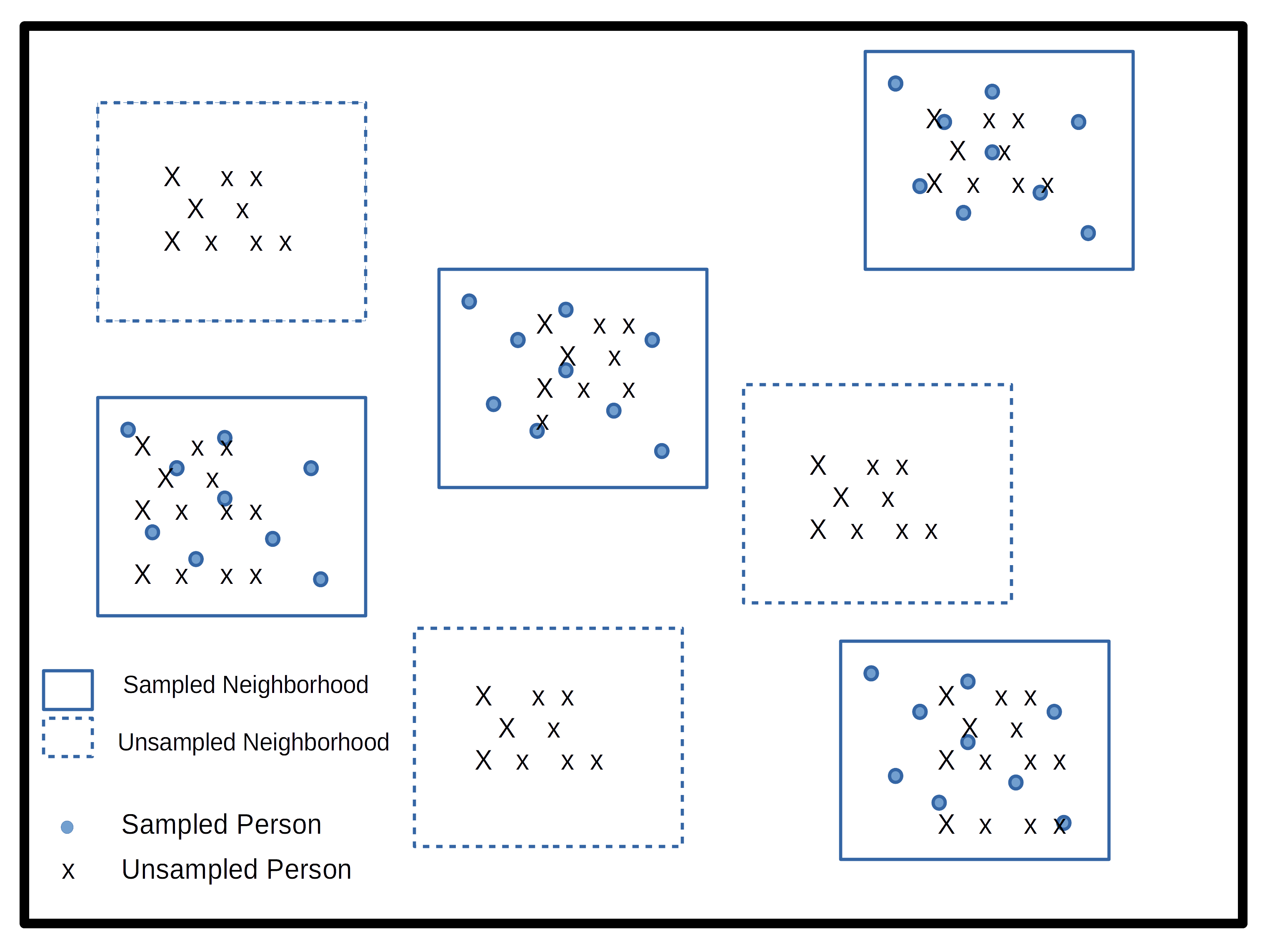
Here’s a picture of a one-stage design, from week 2. Some neighborhoods are sampled (solid lines) and some aren’t (dotted lines), and within the sampled neighborhoods, some people are sampled (circles) and some aren’t (X’s).

Multistage sampling

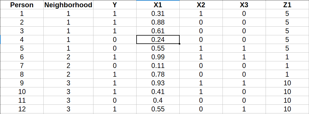
The data from a design like this look like the table below: 12 people in three neighborhoods, each with an outcome \(Y\) and three individual predictors, \(X_1\) to \(X_3\). There’s also a neighborhood-level variable, \(Z_1\), which is the same for everyone in a neighborhood but differs between neighborhoods. A real example would be the neighborhood poverty rate.

Multilevel data

Multilevel propositions

When a research question involves individuals within some context, it’s a multilevel proposition. Using the data structure above, with an outcome \(Y\) and a predictor \(X\) measured on individuals and a contextual variable \(Z\) measured on neighborhoods:

Multilevel data structure

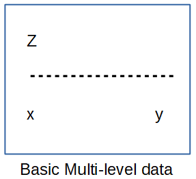
1. An individual-level (micro) proposition relates \(X\) to \(Y\) for individuals: a person’s education affects their health.

   

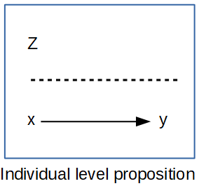
   Micro-level proposition

2. A macro-level proposition relates \(Z\) to \(Y\) measured on places, as in week 6: metros with higher poverty rates have higher mortality rates. This is an ecological analysis, because we see no variation within places.

   

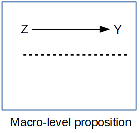
   Macro-level proposition

3. A multilevel proposition uses both \(X\) and \(Z\) to understand an individual outcome: for people with the same education, does living in a high-poverty area affect health? We’re usually looking for the net effect of \(Z\) after accounting for \(X\).

   

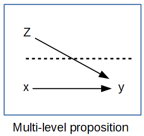
   Multilevel proposition

4. A cross-level interaction asks whether the effect of \(X\) depends on \(Z\): people with less education and who live in high-poverty areas have higher risk of poor health. The important word is and.

   

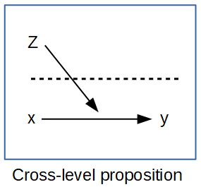
   Cross-level interaction

The multilevel model

Starting from ANOVA

The basic multilevel model is a direct analog of the analysis of variance. In an ANOVA, the mean of group \(j\) is

\[E(y_j) = \mu + u_j\]

the overall mean \(\mu\) plus a deviation \(u_j\) for each group. With 3 to 5 groups, that’s efficient, and the \(u_j\) are fixed effects, estimated relative to a reference group. With dozens or hundreds of groups, it gets awkward. People in 10% of U.S. counties would mean over 300 groups and 300 parameters, and why compare every county to one arbitrary reference county?

The multilevel model estimates the overall mean \(\mu\) and treats the group deviations as draws from a normal distribution, \(u_j \sim N(0, \sigma^2_u)\). That’s a random effect. You can still recover a mean for every group, but the model has (technically) two parameters, \(\mu\) and \(\sigma^2_u\). Add individual predictors and you have a mixed model, with fixed effects \(\beta_k\) and a random effect \(u_j\):

\[y_{ij} = \beta_{0j} + \sum_k \beta_k x_{kij} + e_{ij}\] \[\beta_{0j} = \beta_0 + u_j\]

The \(u_j\) are the random intercepts. Software rarely prints them, because there can be many, but every package reports their variance, \(\sigma^2_u\).

Components of variation

With a normally distributed outcome, there are two sources of variation: the person-level residual \(e_{ij}\) with variance \(\sigma^2_e\), and the between-group variation \(u_j\) with variance \(\sigma^2_u\). The total variance is \(\sigma^2_y = \sigma^2_e + \sigma^2_u\), and the intraclass correlation is

\[\text{ICC} = \frac{\sigma^2_u}{\sigma^2_u + \sigma^2_e}\]

The ICC is the share of the variance that’s between groups, and it’s also the correlation between two randomly chosen people in the same randomly chosen group: how similar you are, on average, to one of your neighbors. It runs from 0 to 1. Notice what it is and isn’t. It’s a way of partitioning the variance under this model: add predictors and it changes. It isn’t the share of the outcome caused by place. Metros differ in BMI partly because different kinds of people live in them, and the empty model’s ICC lumps that in with anything about the places themselves. An ICC of 0.5 is very large, and 0.01 means you’re barely more like your neighbors than like a stranger.

When to use fixed effects and when to use random effects

1. Use fixed effects (dummy variables) when each group is unique, you want conclusions about each one, and you know all of them in advance: sex, race and ethnicity, the four census regions.
2. Use random effects when the groups can be thought of as a sample from a (real or hypothetical) population of groups, like metro areas, schools or counties, and you want conclusions about that population. With more than 10 or so groups, you’re probably not interested in every pairwise difference, and the model has many parameters you don’t care about.

Week 10 added a third consideration: a random effects model assumes the group effects are unrelated to the predictors. Centering, below, is how we deal with that.

Multilevel data sources

Not every question is multilevel, and not every data set can support a multilevel analysis. Public-use files that identify a geographic level include the ECLS-K (school identifiers), the BRFSS (metro areas), the ACS (PUMA, metro and state), and the Demographic and Health Surveys (regions, and GPS coordinates for clusters). Others, like NHANES, the NHIS, Add Health, the PSID and the NLSY, identify geography only in restricted-use files.

Setup

lme4 fits multilevel models (Bates et al. 2015), and WeMix fits them with survey weights (Bailey et al. 2023). get_mmsa_context() downloads metro-level characteristics from the ACS.

library(tidyverse)
library(here)
library(lme4)
library(WeMix)
library(modelsummary)
library(sparkscolors)  # pak::pak("coreysparks/sparkscolors"), UTSA colors

source(here("R", "get_mmsa.R"))
source(here("R", "recode_mmsa.R"))
source(here("R", "get_mmsa_context.R"))

The data: people in metro areas

Contextual data for metro areas

The BRFSS SMART file identifies the metro area each respondent lives in. For the largest metros, like Dallas-Fort Worth and New York, it identifies metropolitan divisions, which are pieces of a metro area. The ACS publishes data for metro areas but not for divisions, so get_mmsa_context() downloads the ACS estimates for every county and adds them up to metro areas and divisions, using the Census Bureau’s file that says which counties belong to which. Every rate is computed from summed counts, not by averaging county rates. Mismatched geographies like this are one of the most common, and most frustrating, problems in contextual research, and you’ll run into them.

context <- get_mmsa_context()
head(context)

#> # A tibble: 6 × 5
#>   mmsa  pct_poverty pct_unemp pct_hisp pct_ba
#>   <chr>       <dbl>     <dbl>    <dbl>  <dbl>
#> 1 10100        10.4      3.24     4.20   32.8
#> 2 10140        14.1      6.61    10.8    17.6
#> 3 10180        13.2      2.73    24.0    26.2
#> 4 10220        12.6      3.52     6.29   29.7
#> 5 10300        11.6      5.40     8.75   22.3
#> 6 10380        47.4     11.8     97.6    24.4

Scaling higher-level variables

Interpreting a contextual variable on its natural scale is often unhelpful. A one-point change in the poverty rate is a small difference, and a change from 0 to 1 in a proportion is from 0% to 100%, which no place experiences. The usual practice is to z-score contextual variables, \(z = (x - \bar x)/\text{sd}(x)\), so a one-unit change compares a place one standard deviation above average to an average place. And because the variable describes places, the mean and standard deviation should be computed across places, not across people. Otherwise, big metros, with many respondents, count more than small ones.

brfss <- get_mmsa() |>
  recode_mmsa() |>
  mutate(mmsa = as.character(mmsa)) |>
  filter(!is.na(bmi), bmi < 70, !is.na(educ), !is.na(race_eth))

# z-score the contextual variables across the metros in the BRFSS
context_z <- context |>
  filter(mmsa %in% brfss$mmsa) |>
  mutate(across(c(pct_poverty, pct_unemp, pct_ba), \(x) as.numeric(scale(x)),
                .names = "z_{.col}"))

brfss <- brfss |>
  left_join(context_z, by = "mmsa") |>
  mutate(college = as.numeric(educ == "College graduate"),
         age_c = (age80 - 50) / 10)

brfss |>
  summarise(people = n(), metros = n_distinct(mmsa),
            smallest = min(table(mmsa)), largest = max(table(mmsa)))

#> # A tibble: 1 × 4
#>   people metros smallest largest
#>    <int>  <int>    <int>   <int>
#> 1 203242    126      440   10773

Before any model, sort the variables by level. Level 1 is people, and level 2 is metro areas. Each person belongs to exactly one metro.

Variable	Level	Varies…
bmi (the outcome)	1 (person)	between people, within and across metros
college, age_c, female, race_eth	1 (person)	between people in the same metro
college_mean (share of a metro’s respondents who are college graduates)	2 (metro)	only between metros; everyone in a metro has the same value
z_pct_poverty, z_pct_unemp, z_pct_ba (from the ACS)	2 (metro)	only between metros

A level-2 variable can only explain differences between metros, because it doesn’t vary within them.

NoteCode explanation: across() with .names

across(c(pct_poverty, pct_unemp, pct_ba), \(x) as.numeric(scale(x)), .names = "z_{.col}") z-scores three columns at once. scale() subtracts the mean and divides by the standard deviation, and returns a matrix, so as.numeric() turns it back into a plain vector. .names = "z_{.col}" keeps the original columns and adds new ones, with {.col} replaced by each original name: z_pct_poverty, z_pct_unemp and z_pct_ba.

The outcome this week is BMI. I’ve centered age at 50 and divided by 10, so its coefficient is the change per decade and the intercept describes a 50-year-old.

How much variation is between metro areas?

The empty model

Start with no predictors at all, just a random intercept for each metro. The formula (1 | mmsa) means “an intercept for each value of mmsa, drawn from a normal distribution.”

fit0 <- lmer(bmi ~ 1 + (1 | mmsa), data = brfss)
summary(fit0)

#> Linear mixed model fit by REML ['lmerMod']
#> Formula: bmi ~ 1 + (1 | mmsa)
#>    Data: brfss
#> 
#> REML criterion at convergence: 1328714
#> 
#> Scaled residuals: 
#>     Min      1Q  Median      3Q     Max 
#> -2.6988 -0.6788 -0.1601  0.4949  6.7277 
#> 
#> Random effects:
#>  Groups   Name        Variance Std.Dev.
#>  mmsa     (Intercept)  0.4375  0.6615  
#>  Residual             40.3686  6.3536  
#> Number of obs: 203242, groups:  mmsa, 126
#> 
#> Fixed effects:
#>             Estimate Std. Error t value
#> (Intercept) 28.49566    0.06156   462.9

vc0 <- as.data.frame(VarCorr(fit0))
icc0 <- vc0$vcov[1] / sum(vc0$vcov)

The standard deviation of the metro intercepts is 0.66 BMI points, and the person-level residual standard deviation is 6.35. So the ICC is 0.011: about 1.1% of the variation in BMI is between metro areas. That’s small, and typical for individual health outcomes across large places. Most of the variation in BMI is between people, not places. But a 1% ICC isn’t nothing, and it doesn’t mean context is unimportant: a standard deviation of 0.66 across metros means the metros in the middle 95% span about 2.6 BMI points, which matters for a population.

TipReading the result: a right and a wrong interpretation

Right: “In a model with no predictors, about 1.1% of the variance in BMI is between metro areas, and the rest is between people within metros.”

Wrong: “Where people live causes 1.1% of the differences in BMI.” The ICC is a split of the variance, not a causal share. Part of the between-metro variance comes from who lives in each metro (their age, education and so on), and part from anything about the places; the empty model can’t tell those apart.

NoteCode explanation: VarCorr()

VarCorr() pulls the variance components out of a fitted lmer() model, and as.data.frame() turns them into a table with one row per component: vcov is the variance and sdcor the standard deviation. The first row is the metro intercepts and the last is the residual.

The metro intercepts, and shrinkage

The model doesn’t estimate the metro intercepts as parameters, but you can get their predicted values after the fact, which lme4 calls the conditional modes (you’ll also see them called BLUPs or empirical Bayes estimates).

re0 <- as.data.frame(ranef(fit0, condVar = TRUE)) |>
  left_join(count(brfss, mmsa, place), by = c("grp" = "mmsa"))

re0 |>
  mutate(grp = fct_reorder(grp, condval)) |>
  ggplot(aes(x = condval, y = grp)) +
  geom_vline(xintercept = 0, colour = utsa_cols("smoke")) +
  geom_pointrange(aes(xmin = condval - 1.96 * condsd, xmax = condval + 1.96 * condsd),
                  colour = utsa_cols("midnight"), size = 0.1) +
  labs(x = "Deviation from overall mean BMI", y = "Metro area") +
  theme(axis.text.y = element_blank(), panel.grid.major.y = element_blank())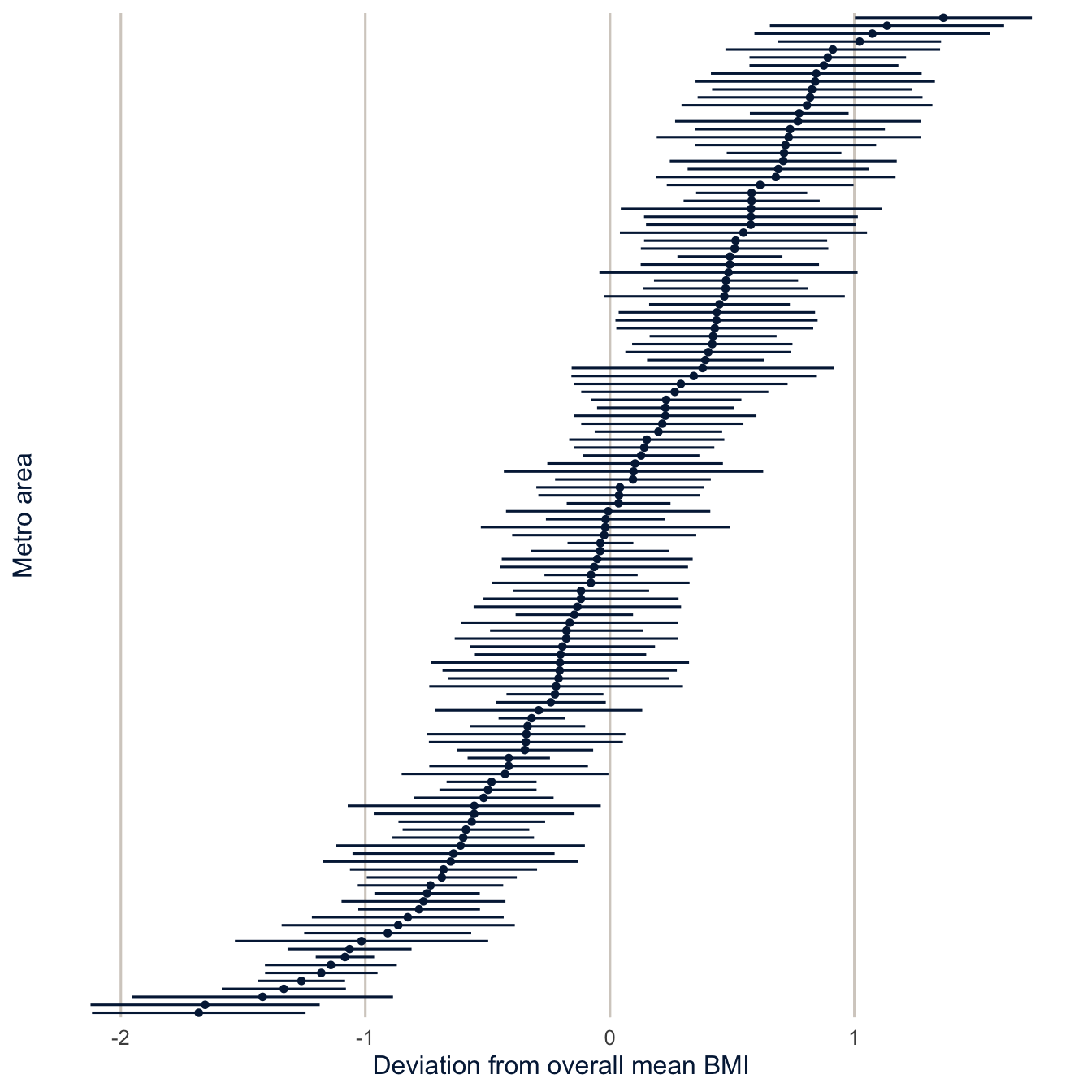

Figure 12.1: Predicted metro deviations from the overall mean BMI, with 95% intervals, from the empty model.

ranef(fit0, condVar = TRUE) gets the predicted metro intercepts and their uncertainty; as a data frame, condval is each prediction, condsd its standard deviation, and grp the metro ID. count(brfss, mmsa, place) counts respondents per metro (keeping the name), and fct_reorder(grp, condval) sorts the metros by their predicted deviation for the plot.

Each point is one metro’s predicted deviation from the overall mean. The predictions are shrunk toward zero, more so for metros with few respondents. If a metro has 500 respondents, its sample mean is noisy, and the model pulls it toward the overall mean; with 10,000 respondents, the sample mean speaks for itself. This is called partial pooling. Two extremes are possible: “no pooling” would use each metro’s own sample mean, however noisy, and “complete pooling” would ignore the metros and use the overall mean for everyone. The random intercept model does something in between, and how far it leans toward the overall mean depends on how much information each metro has. Small metros are pulled more toward the overall pattern; big ones mostly keep their own means. This is one of the real advantages of the multilevel model: it borrows strength from the other groups to make better estimates for the small ones.

re0 |>
  left_join(brfss |> group_by(mmsa) |> summarise(raw = mean(bmi) - fixef(fit0)[1]),
            by = c("grp" = "mmsa")) |>
  mutate(size = if_else(n < median(n), "Smaller samples", "Larger samples")) |>
  group_by(size) |>
  summarise(sd_raw_deviation = sd(raw), sd_predicted = sd(condval))

#> # A tibble: 2 × 3
#>   size            sd_raw_deviation sd_predicted
#>   <chr>                      <dbl>        <dbl>
#> 1 Larger samples             0.640        0.610
#> 2 Smaller samples            0.748        0.651

The raw metro means vary more than the predictions, and the difference is biggest for the metros with smaller samples.

Individual predictors

fit1 <- lmer(bmi ~ college + age_c + I(age_c^2) + female + race_eth + (1 | mmsa), data = brfss)
anova(fit0, fit1)

#> Data: brfss
#> Models:
#> fit0: bmi ~ 1 + (1 | mmsa)
#> fit1: bmi ~ college + age_c + I(age_c^2) + female + race_eth + (1 | mmsa)
#>      npar     AIC     BIC  logLik -2*log(L)  Chisq Df Pr(>Chisq)    
#> fit0    3 1328716 1328747 -664355   1328710                         
#> fit1   11 1318827 1318939 -659403   1318805 9905.1  8  < 2.2e-16 ***
#> ---
#> Signif. codes:  0 '***' 0.001 '**' 0.01 '*' 0.05 '.' 0.1 ' ' 1

The likelihood ratio test says the individual predictors explain a lot, as you’d expect. (anova() refits both models by maximum likelihood before comparing them, because the default REML fits can’t be compared when the fixed effects differ.)

Centering

Why centering matters in multilevel models

In week 10, we split poverty into a within-child part and a between-child part. The same issue comes up whenever a person-level predictor varies both within and between groups. College graduation varies across people within every metro, and the share of college graduates varies across metros, from 24% to 64% of respondents. A single coefficient on college mixes the two, just as the random effects coefficient on poverty did. Enders and Tofighi (2007) lay out the options.

Here’s a small example first. Two metros, three people each, with college coded 1 for college graduates:

Person	Metro	college	Metro mean, \(\bar x_j\)	Group-mean centered, \(x_{ij} - \bar x_j\)	Grand-mean centered, \(x_{ij} - \bar x\)
1	A	1	0.67	0.33	0.50
2	A	1	0.67	0.33	0.50
3	A	0	0.67	−0.67	−0.50
4	B	1	0.33	0.67	0.50
5	B	0	0.33	−0.33	−0.50
6	B	0	0.33	−0.33	−0.50

The grand mean is \(\bar x = 0.5\) (three of six people). Look at persons 1 and 4, both college graduates. Their grand-mean-centered values are the same, 0.5, because they’re compared with everyone. But their group-mean-centered values differ: person 1 is a college graduate in a metro where most people are (0.33 above the metro mean), and person 4 is a college graduate in a metro where most people aren’t (0.67 above it). The group-mean-centered variable compares each person with others in the same metro. The metro mean, 0.67 or 0.33, is a separate, between-metro comparison. Including both in the model keeps the two relationships from being blended together.

1. No centering, or grand-mean centering (subtracting the overall mean): the coefficient on \(x_{ij}\) is a blend of the within- and between-group relationships.
2. Group-mean centering (subtracting each group’s mean, \(x_{ij} - \bar x_j\)), and adding the group mean \(\bar x_j\) as a level-2 predictor: the coefficient on the centered variable is the pure within-group effect, and the coefficient on \(\bar x_j\) is the between-group effect.
3. Grand-mean centering plus the group mean: the coefficient on \(x_{ij}\) is the within-group effect, and the coefficient on \(\bar x_j\) is the contextual effect, how much more the group mean matters than the individual value. The contextual effect is the between effect minus the within effect.

brfss <- brfss |>
  group_by(mmsa) |>
  mutate(college_mean = mean(college),
         college_cwc = college - college_mean) |>      # centered within cluster
  ungroup() |>
  mutate(college_cgm = college - mean(college))       # centered at the grand mean

fit_raw <- lmer(bmi ~ college + age_c + I(age_c^2) + female + race_eth + (1 | mmsa), data = brfss)
fit_cwc <- lmer(bmi ~ college_cwc + college_mean + age_c + I(age_c^2) + female + race_eth + (1 | mmsa),
                data = brfss)
fit_cgm <- lmer(bmi ~ college_cgm + college_mean + age_c + I(age_c^2) + female + race_eth + (1 | mmsa),
                data = brfss)

modelsummary(list("Uncentered" = fit_raw, "Group-mean centered" = fit_cwc,
                  "Grand-mean centered + mean" = fit_cgm),
             coef_map = c(college = "College graduate", college_cwc = "College (within metro)",
                          college_cgm = "College (grand-mean centered)",
                          college_mean = "Metro share college graduates"),
             gof_map = c("nobs", "aic"), statistic = "std.error")

	Uncentered	Group-mean centered	Grand-mean centered + mean
College graduate	-1.067
	(0.028)
College (within metro)		-1.061
		(0.028)
College (grand-mean centered)			-1.061
			(0.028)
Metro share college graduates		-7.014	-5.954
		(0.509)	(0.510)
Num.Obs.	203242	203242	203242
AIC	1318873.4	1318782.1	1318782.1

In the table, coef_map both picks which coefficients to show and gives them readable labels; any coefficient not listed is left out.

Being a college graduate is associated with a BMI 1.06 points lower than other people in the same metro. That’s the within effect. The between effect is -7.01 for a change in the metro share from 0 to 1, so a metro where 10 percentage points more of the respondents are college graduates has an average BMI about 0.7 points lower. The contextual effect, -5.95, is the difference between the two (-7.01 − (-1.06) = -5.95): living in a more educated metro is associated with lower BMI beyond what you’d expect from the education of the individuals who live there. Notice that the uncentered coefficient, -1.07, is almost exactly the within effect here. With so many people per metro, the within-metro comparison dominates.

Is the contextual effect causal? Not necessarily. More educated metros differ from less educated ones in many ways (income, the built environment, the age and migration history of the population), and the metro share of college graduates stands in for all of them. It’s a description of how BMI is patterned across places, and a starting point for asking why.

Random slopes

Letting the effect of education differ across metros

So far, every metro has its own intercept but the same slope for college graduation. A random slope lets the within-metro association differ too. Get comfortable with random intercepts before this step: a random intercept lets each metro’s baseline differ, and a random slope also lets each metro’s relationship between education and BMI differ:

\[y_{ij} = \beta_{0j} + \beta_{1j} x_{ij} + \cdots + e_{ij}\] \[\beta_{0j} = \beta_0 + u_{0j}, \qquad \beta_{1j} = \beta_1 + u_{1j}\]

The model now estimates the variance of the slopes and the correlation between intercepts and slopes. In lmer(), the syntax is (1 + college_cwc | mmsa).

fit_rs <- lmer(bmi ~ college_cwc + college_mean + age_c + I(age_c^2) + female + race_eth +
                 (1 + college_cwc | mmsa), data = brfss)
VarCorr(fit_rs)

#>  Groups   Name        Std.Dev. Corr  
#>  mmsa     (Intercept) 0.38593        
#>           college_cwc 0.31708  0.167 
#>  Residual             6.19945

anova(fit_cwc, fit_rs, refit = FALSE)

#> Data: brfss
#> Models:
#> fit_cwc: bmi ~ college_cwc + college_mean + age_c + I(age_c^2) + female + race_eth + (1 | mmsa)
#> fit_rs: bmi ~ college_cwc + college_mean + age_c + I(age_c^2) + female + race_eth + (1 + college_cwc | mmsa)
#>         npar     AIC     BIC  logLik -2*log(L)  Chisq Df Pr(>Chisq)    
#> fit_cwc   12 1318782 1318905 -659379   1318758                         
#> fit_rs    14 1318755 1318898 -659363   1318727 31.107  2  1.759e-07 ***
#> ---
#> Signif. codes:  0 '***' 0.001 '**' 0.01 '*' 0.05 '.' 0.1 ' ' 1

NoteCode explanation: comparing random effects structures

anova(fit_cwc, fit_rs, refit = FALSE) compares the models with and without the random slope. When the models have the same fixed effects and differ only in their random effects, compare the REML fits directly (refit = FALSE). The test is conservative, because the null hypothesis (a slope variance of zero) is on the boundary of the possible values; the usual fix is to halve the p-value.

The standard deviation of the college slopes across metros is 0.32, around an average slope of -1.02. So in most metros, college graduates have lower BMI than their neighbors by somewhere between about 0.4 and 1.7 points, and the likelihood ratio test says that variation is real.

Explaining the slope variation: a cross-level interaction

If the college gap in BMI differs across metros, it’s natural to ask whether it’s related to something about the metros. Interacting a person-level variable with a metro-level variable is the cross-level interaction from the beginning of the document: it asks whether the slopes differ systematically with a characteristic of the metro, rather than just at random.

fit_cli <- lmer(bmi ~ college_cwc * z_pct_poverty + college_mean + age_c + I(age_c^2) + female +
                  race_eth + (1 + college_cwc | mmsa), data = brfss)
summary(fit_cli)$coefficients[c("college_cwc", "z_pct_poverty", "college_cwc:z_pct_poverty"), ]

#>                              Estimate Std. Error    t value
#> college_cwc               -1.01229167 0.04275844 -23.674664
#> z_pct_poverty             -0.10508736 0.04078461  -2.576643
#> college_cwc:z_pct_poverty  0.07463826 0.04016800   1.858152

The interaction is 0.075. In a metro with a poverty rate one standard deviation above average, the college gap in BMI is that much smaller in absolute value. The estimate is 1.9 standard errors from zero, which is suggestive but not convincing, and it’s small next to the slope standard deviation of 0.32. Metro poverty explains little of the variation in the college gap. Remember who the reference is in each term: college_cwc is the gap in an average-poverty metro, and z_pct_poverty is the poverty association for someone at their metro’s mean level of college education.

Diagnostics

The model assumes normal residuals at both levels. Check the person-level residuals against the fitted values, and the metro intercepts and slopes against a normal distribution.

as.data.frame(ranef(fit_rs)) |>
  mutate(term = if_else(term == "(Intercept)", "Intercept", "College slope")) |>
  ggplot(aes(sample = condval)) +
  stat_qq(colour = utsa_cols("midnight")) +
  stat_qq_line(colour = utsa_cols("orange")) +
  facet_wrap(~term, scales = "free_y") +
  labs(x = "Normal quantile", y = "Predicted random effect")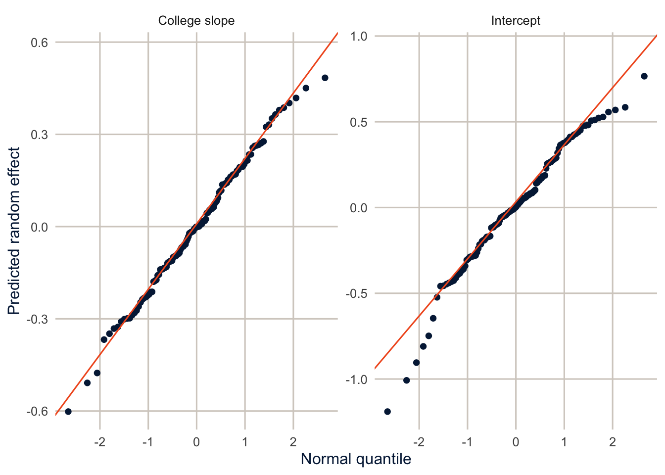

Figure 12.2: Normal quantile plots of the predicted metro intercepts and college slopes from the random slope model.

stat_qq() plots the sorted values against the quantiles of a normal distribution, and stat_qq_line() adds the line they’d follow if they were exactly normal.

The random effects are close to normal, with a few metros out in the tails. BMI itself is right-skewed, so the person-level residuals are too. With over 200,000 people, that doesn’t threaten the fixed effects, but it would be worth trying log BMI in a real analysis.

Survey weights in multilevel models

Why lmer() can’t use sampling weights

Every multilevel model above ignored the BRFSS weights. You might think lmer(..., weights = mmsawt) would fix that. It doesn’t. In lmer(), as in lm(), the weights argument means precision weights: an observation with weight 2 is treated as having half the residual variance, as if it were the average of two measurements. That’s a different thing from a sampling weight, which says how many people in the population a respondent represents. Using sampling weights as precision weights gives wrong standard errors and, in a multilevel model, wrong variance components.

The right approach is pseudo-maximum likelihood with weights at each level (Pfeffermann et al. 1998; Rabe-Hesketh and Skrondal 2006). A two-level model needs two weights: a level-2 weight for the probability that the group was sampled, and a level-1 weight for the probability that a person was sampled given that their group was. In the BRFSS, metro areas aren’t sampled (every metro with enough respondents is included), so the level-2 weight is 1 for every metro, and the level-1 weight is the person weight. Be clear about what that weight of 1 does and doesn’t mean. It says no metro was more likely than another to be chosen at random. It doesn’t say the metros in the file represent all U.S. metros: a metro is in the SMART file only if it had enough respondents, which favors larger metros. So conclusions about “metros” here are about the metros that meet CDC’s reporting rules, not every metro in the country. In the ECLS-K, schools are sampled, and both weights matter. There’s a further complication: in a multilevel model, the scale of the level-1 weights affects the variance components, so different methods of rescaling the weights within groups give different answers, and Rabe-Hesketh and Skrondal (2006) discuss which to prefer.

Weighted multilevel models with WeMix

WeMix fits linear and generalized linear multilevel models with weights at each level, and its standard errors are robust (sandwich) standard errors.

brfss_wm <- brfss |>
  mutate(w1 = mmsawt, w2 = 1) |>
  select(bmi, college_cwc, college_mean, age_c, female, mmsa, w1, w2) |>
  as.data.frame()

fit_wm <- mix(bmi ~ college_cwc + college_mean + age_c + female + (1 | mmsa),
              data = brfss_wm, weights = c("w1", "w2"))
fit_unw <- lmer(bmi ~ college_cwc + college_mean + age_c + female + (1 | mmsa), data = brfss_wm)

NoteCode explanation: mix()

1. The formula uses lme4 syntax.
2. weights = c("w1", "w2") names the weight columns, starting at level 1 and going up. By default, mix() expects unconditional weights at level 1 (the overall weight for each person, which is what the BRFSS gives you) and works out the conditional ones by dividing by the level-2 weight. With w2 = 1, they’re the same.
3. mix() wants a plain data frame, not a tibble, and it’s much slower than lmer(), which is why the chunk is cached.

tibble(term = names(fixef(fit_unw)),
       unweighted = fixef(fit_unw),
       se_unweighted = sqrt(diag(vcov(fit_unw))),
       weighted = fit_wm$coef[names(fixef(fit_unw))],
       se_weighted = fit_wm$SE[names(fixef(fit_unw))]) |>
  knitr::kable(digits = 3)

term	unweighted	se_unweighted	weighted	se_weighted
(Intercept)	31.589	0.242	31.479	0.303
college_cwc	-0.974	0.028	-1.021	0.062
college_mean	-6.896	0.528	-6.807	0.660
age_c	0.019	0.008	0.221	0.017
female	0.012	0.028	-0.057	0.069

The weighted and unweighted estimates are similar for the education terms, but not for age, which is 0.02 unweighted and 0.22 weighted. I left the squared age term out of this model to keep it quick, so it’s misspecified: BMI rises and then falls with age, and a straight line can’t follow that. The weights give younger adults, who are underrepresented in the BRFSS, more influence, which changes which part of the curve the line fits. Weighting makes the biggest difference when the model is wrong, and comparing weighted and unweighted estimates is a useful check on the specification. The weighted standard errors are larger, about 2.2 times as large at the median. That’s the same pattern as week 2: unequal weights cost precision, and an analysis that ignores them is overconfident. The weighted metro-level variance is 0.258, compared with 0.161 unweighted.

TipFew groups? Consider a Bayesian model

Multilevel models estimate the variance of the group effects from the groups, so with only a handful of groups (fewer than 20 or so), that variance is poorly estimated, and lmer() and glmer() often report it as zero or fail to converge. A Bayesian multilevel model is one option (optional for this course). You have to choose explicit priors, statements of what values the parameters could plausibly take before seeing the data. A weakly informative prior on the variance keeps the estimate away from implausible values like exactly zero, and the brms package makes this easy, with the same syntax as lme4’s. But it doesn’t create information that isn’t there: with few groups, the estimate of the variance still depends heavily on the prior, so you should say what prior you used and check how much the results change with a different one.

library(brms)
fit_bayes <- brm(bmi ~ college_cwc + college_mean + age_c + female + (1 | mmsa),
                 data = brfss, chains = 4, cores = 4)

brms writes and compiles a Stan program behind the scenes, so the first run takes a while, and you’ll need a C++ compiler (Rtools on Windows, from week 1). Gelman and Hill (2007) is the classic applied introduction to this way of thinking.

Summary

Multilevel models put individuals inside places and estimate how much of the variation in an outcome is between places, through the variance of the random intercepts and the ICC. The predicted group effects are shrunk toward the overall mean, more so for small groups. Person-level predictors that vary within and between groups should be split by group-mean centering into within and between parts, as in week 10, and the difference between the two is the contextual effect. Random slopes let the effect of a predictor vary across groups, and cross-level interactions ask whether that variation is related to characteristics of the groups. lmer() can’t use sampling weights; for weighted multilevel models, use WeMix with a weight at each level. Raudenbush and Bryk (2002) and Gelman and Hill (2007) are the standard references.

Homework 12

Due: April 15, before class.

Which version to do. If you’re in DEM 7283, do the version with your own survey data. If you’re in DEM 5283, do either version, and say at the top of your homework which one you did. If your survey can’t support this week’s method, do the version with my data and say so.

Purpose. Fit and interpret multilevel models, keeping the person-level and metro-level comparisons apart.

A satisfactory answer names the two levels; interprets the random intercept variance and the ICC as a split of the variance, not a causal share; interprets within-metro and between-metro terms separately; and says which population of metros the conclusions describe.

With your own survey data

Use the full survey design for every estimate unless a step says otherwise, and report each estimate with a standard error or confidence interval.

This homework needs a grouping variable with enough groups (at least 30 or so). If your survey doesn’t have one, use the BRFSS metro-area data from the chapter.

1. Identify the grouping variable in your data (for example, state, county, metro area or survey cluster), and how many people are in each group.
2. Construct at least one group-level variable, either by aggregating your survey data or by merging contextual data (for example, from the ACS with tidycensus). Explain how you scaled it.
3. Fit a null (random intercept only) model for a continuous outcome.
   1. Report the variance components and the intraclass correlation.
   2. Interpret the ICC in a sentence.
4. Add individual-level predictors, then your group-level variable.
   1. How do the variance components change at each step?
   2. Interpret the coefficient for your group-level variable.
5. Centering. Choose one individual-level predictor and fit the model with it grand-mean centered and then group-mean centered (with the group mean added as a level-2 predictor). How do the coefficients and their interpretations differ?
6. Fit a random slope for one individual-level predictor.
   1. Is there evidence that its association varies across groups? How do you know?
   2. Plot the group-specific slopes.
7. Fit your final model with level-specific weights using WeMix, if your survey supplies them, and compare it with the unweighted model. If your survey doesn’t supply weights at each level, explain what you would need, and what that means for the population your estimates describe.

With my data

What is provided. The BRFSS data brfss with metro context, college_mean, college_cwc and college_cgm, and the models from this chapter.

1. Fit an empty model for the number of poor mental health days in the past month (ment_days), with a random intercept for metro area. Identify the two levels of the data. Interpret the random intercept variance and the ICC, and compare the ICC with BMI’s. Then add the group-mean centered college variable and the metro share of college graduates, and interpret the within-metro and between-metro terms separately, in days. Explain shrinkage in a sentence, using what happens to the predicted intercepts for the smallest metros. Finally, say which population of metro areas your conclusions can reasonably describe.

# YOUR CODE HERE

2. Split age into within-metro and between-metro parts (group-mean center age_c and add the metro mean age) in the BMI model. Is there a contextual effect of a metro’s age structure? What would it mean?

# YOUR CODE HERE

3. Add the z-scored metro unemployment rate (z_pct_unemp) and share of adults with a bachelor’s degree from the ACS (z_pct_ba) to the group-mean centered model. How does the ACS measure of metro education compare with the BRFSS sample share, college_mean?

# YOUR CODE HERE

One solution for exercise 3

fit_acs <- lmer(bmi ~ college_cwc + z_pct_ba + z_pct_unemp + age_c + I(age_c^2) + female +
                  race_eth + (1 | mmsa), data = brfss)
fit_both <- update(fit_acs, . ~ . + college_mean)
modelsummary(list("ACS education" = fit_acs, "ACS and BRFSS" = fit_both),
             gof_map = c("nobs", "aic"))

The ACS share is measured on the whole population, not a sample, so it’s a less noisy measure of metro education, but it’s for adults 25 and older, and the BRFSS share is for adults 18 and older. When both are in the model, they compete for the same between-metro variation.

4. Fit the random slope model with WeMix and compare the variance of the college slopes with the unweighted estimate. (This takes a few minutes.)

# YOUR CODE HERE

Additional resources

• Gelman and Hill (2007), chapters 11 to 13, are the best applied introduction to multilevel models I know of, and their discussion of partial pooling is worth reading twice.
• Enders and Tofighi (2007), “Centering Predictor Variables in Cross-Sectional Multilevel Models”, Psychological Methods, the reference for grand-mean and group-mean centering.
• Bates et al. (2015), “Fitting Linear Mixed-Effects Models Using lme4”, Journal of Statistical Software, explains what lmer() does and how to read its output.
• The Centre for Multilevel Modelling at Bristol has a free online course with modules on everything from variance components to cross-classified models.

Bailey, Paul, Blue Webb, Claire Kelley, Trang Nguyen, and Huade Huo. 2023. WeMix: Weighted Mixed-Effects Models Using Multilevel Pseudo Maximum Likelihood Estimation. https://doi.org/10.32614/CRAN.package.WeMix.

Bates, Douglas, Martin Mächler, Ben Bolker, and Steve Walker. 2015. “Fitting Linear Mixed-Effects Models Using lme4.” Journal of Statistical Software 67 (1): 1–48.

Enders, Craig K., and Davood Tofighi. 2007. “Centering Predictor Variables in Cross-Sectional Multilevel Models: A New Look at an Old Issue.” Psychological Methods 12 (2): 121–38.

Gelman, Andrew, and Jennifer Hill. 2007. Data Analysis Using Regression and Multilevel/Hierarchical Models. Cambridge University Press.

Pfeffermann, Danny, Chris J. Skinner, David J. Holmes, Harvey Goldstein, and Jon Rasbash. 1998. “Weighting for Unequal Selection Probabilities in Multilevel Models.” Journal of the Royal Statistical Society: Series B 60 (1): 23–40.

Rabe-Hesketh, Sophia, and Anders Skrondal. 2006. “Multilevel Modelling of Complex Survey Data.” Journal of the Royal Statistical Society: Series A 169 (4): 805–27.

Raudenbush, Stephen W., and Anthony S. Bryk. 2002. Hierarchical Linear Models: Applications and Data Analysis Methods. 2nd ed. Sage.