library(tidyverse)
library(here)
library(survey)
library(mice)
library(mitools)
library(sparkscolors)  # pak::pak("coreysparks/sparkscolors"), UTSA colors

source(here("R", "get_mmsa.R"))
source(here("R", "recode_mmsa.R"))Week 9: Missing Data and Multiple Imputation
Introduction
Every time we ask a question on a survey, there are reasons we might not get an answer, and every model you’ve fit so far this semester has quietly dealt with that by dropping anyone with a missing value on any variable in the model. That’s called listwise deletion, or complete-case analysis, and it is the default in R, Stata, SAS and everything else. Sometimes it’s fine. Often it throws away a lot of people, and it changes who contributes to the estimate: if the people it throws away are different from the people it keeps, the results can be biased too. Whether they actually are depends on what you’re estimating and on why the data are missing, which is what the first part of this chapter is about.
This week covers why data go missing, what kinds of missingness we can and can’t live with, the easy ways to fill in missing values (which are bad ways), and multiple imputation, which is the method I’d recommend for most demographic analyses. I’ll pay particular attention to doing multiple imputation with survey data, because the usual textbook example drops the design, and you’ve spent eight weeks learning not to do that.
NoteThis week at a glance
The question. How does fair or poor health differ by education and income among adults in Texas metro areas, when a sixth of them didn’t report their income?
By the end of this week you should be able to
- distinguish MCAR, MAR and MNAR with an example, and explain why the data can show that values are not MCAR but can never show that they are MAR;
- explain why filling in each missing value once understates uncertainty, and what Rubin’s rules add;
- run a multiple imputation that keeps the survey design, and compare it with a complete-case analysis without claiming that either proves the missingness assumption.
Before you begin. You need the survey design and svyglm() from weeks 2 and 3, and the map() and across() patterns from week 2 and week 1.
Required and optional. Everything is required except the details of the von Hippel formula for the number of imputations; the idea that more imputations give more stable standard errors is enough.
Setup
The mice package does the imputation (Buuren and Groothuis-Oudshoorn 2011), and mitools combines the results across imputed data sets. The survey package can work directly with a list of imputed data sets, so the design stays in the analysis.
Why data go missing
Reasons for missing data
Survey methodologists sort missing data by how much of a person’s information is missing.
- Total nonresponse. The sampled person never participates: they refuse, they’re never home, they’re too ill. We usually have nothing on them but the sampling frame information, and the survey weights are built to account for them (that was week 2’s raking story).
- Noncoverage. The person was never in the sampling frame at all, like people without phones in a phone survey. This is also handled, as well as it can be, by the weights.
- Item nonresponse. The person participates but doesn’t answer a particular question. They refuse, they say “I don’t know,” they give an answer that doesn’t make sense, or the interviewer skips the question. This is what imputation is for.
- Partial nonresponse. Somewhere in between: someone starts the interview and quits partway, or answers one wave of a panel study and not the next. Agencies handle this with weights (dropping the partial cases and reweighting the rest) or by imputing the missing items.
This week is about item nonresponse, because it’s the kind you have to deal with. Income is the classic example. People don’t like to tell a stranger on the phone how much money they make, but they’re usually happy to tell you their age, education, and whether they own their home, and those things tell us a lot about their income.
Types of missing data
Little and Rubin (2019) gave us the vocabulary everyone uses. The three types are about what the probability of being missing depends on. I’ll use one example for all three: income, missing for some BRFSS respondents.
- Missing completely at random (MCAR). Whether a value is missing has nothing to do with anything about the person, observed or not. Income would be MCAR if, say, a random batch of interviewers skipped the question by mistake. Complete-case analysis is unbiased under MCAR; it just loses precision.
- Missing at random (MAR). Whether a value is missing depends on other things we observed about the person, but not on the missing value itself once we take those into account. Income is MAR if older and less educated respondents are less likely to report it, but among people of the same age and education, the chance of reporting doesn’t depend on how much they earn. The name is unfortunate, because MAR isn’t random in any everyday sense: the missingness can depend strongly on observed variables.
- Missing not at random (MNAR). Whether a value is missing depends on the value itself, even after accounting for everything we observed. Income is MNAR if, among people of the same age and education, those with the highest (or lowest) incomes are least likely to report them because of what their incomes are.
MCAR and MAR are called ignorable, because the methods below can recover unbiased estimates without modeling why the data are missing. MNAR is non-ignorable, and handling it requires assumptions you can’t check with the data you have.
Don’t read that as “complete-case analysis is always biased unless the data are MCAR,” though. It depends on what you’re estimating. For example, if you’re estimating a regression, and whether a value is missing depends only on the predictors in the model (not on the outcome), the complete-case coefficients are still unbiased, even though the data aren’t MCAR. What complete-case analysis always does is change who contributes to the estimate, and you have to think through whether that matters for your question.
What the computer does
Left to itself, software does one of two things. Listwise deletion drops the whole case if any variable in the model is missing. Pairwise deletion drops a case only from the calculations that need the missing variable, so a correlation matrix might be built from different people in each cell. Both give you fewer cases, and neither fixes bias unless the data are MCAR.
The data
I’ll use the Texas metro areas from the 2024 BRFSS, which keeps the imputation fast enough to run in class. Because the BRFSS strata are nested within states, the Texas respondents carry their full design (you saw this in week 2). The outcome is fair or poor self-rated health, and the predictors are income, education, race and ethnicity, age, sex, smoking, BMI and insurance.
tx <- get_mmsa() |>
  recode_mmsa() |>
  filter(texas, !is.na(badhealth)) |>
  mutate(place = factor(place),
         log_wt = log(mmsawt),
         # income and education as ordered numeric codes (see below)
         income_n = as.integer(income),
         educ_n = as.integer(educ))

analysis_vars <- c("badhealth", "income_n", "educ_n", "race_eth", "agec",
                   "female", "smoke", "bmi", "insured")

tx |>
  summarise(across(all_of(analysis_vars), \(x) mean(is.na(x)))) |>
  pivot_longer(everything(), names_to = "variable", values_to = "share_missing") |>
  arrange(desc(share_missing)) |>
knitr::kable(digits = 3)| variable | share_missing |
|---|---|
| income_n | 0.205 |
| bmi | 0.119 |
| smoke | 0.085 |
| insured | 0.049 |
| race_eth | 0.028 |
| educ_n | 0.007 |
| badhealth | 0.000 |
| agec | 0.000 |
| female | 0.000 |
NoteCode explanation: counting missing values with
across()
across(all_of(analysis_vars), ...)applies the same function to every column named inanalysis_vars.all_of()says “these names are in a character vector,” which is how you handacross()a list of columns you’ve stored ahead of time.\(x) mean(is.na(x))is an anonymous function (week 2’s\(d)again).is.na(x)isTRUEwherexis missing, and the mean of aTRUE/FALSEvector is the share that areTRUE.pivot_longer()turns the one-row result into one row per variable, which is easier to read and sort.
Income is missing for 20.5% of respondents, which is typical for the BRFSS, and BMI for 11.9%. Put all nine variables in one model, and complete-case analysis keeps 5,099 of the 7,509 respondents. We’d lose 32% of the sample before estimating anything.
The easy ways, which are the bad ways
Mean imputation
The simplest fix is to replace every missing value with the mean of the observed values. Here it is for BMI.
bmi_mean_imp <- if_else(is.na(tx$bmi), mean(tx$bmi, na.rm = TRUE), tx$bmi)

tibble(version = c("Observed values only", "Mean imputed"),
       mean = c(mean(tx$bmi, na.rm = TRUE), mean(bmi_mean_imp)),
       median = c(median(tx$bmi, na.rm = TRUE), median(bmi_mean_imp)),
       variance = c(var(tx$bmi, na.rm = TRUE), var(bmi_mean_imp))) |>
knitr::kable(digits = 2)| version | mean | median | variance |
|---|---|---|---|
| Observed values only | 28.49 | 27.41 | 42.99 |
| Mean imputed | 28.49 | 28.34 | 37.86 |
if_else(is.na(tx$bmi), mean(...), tx$bmi) keeps each observed BMI and replaces each missing one with the mean of the observed values. var() is the variance.
The mean doesn’t change (it can’t), the median barely moves, but the variance drops by 12%. Everyone who was missing now sits exactly at the mean, which piles them up in the middle of the distribution and makes BMI look less variable than it is. Any regression coefficient involving BMI will be biased toward zero, and every standard error will be too small, because the model thinks it has 895 real observations at the mean.
tibble(Observed = tx$bmi, `Mean imputed` = bmi_mean_imp) |>
  pivot_longer(everything(), names_to = "version", values_to = "bmi") |>
  filter(!is.na(bmi), bmi < 60) |>
  ggplot(aes(x = bmi, colour = version, linetype = version)) +
  geom_freqpoly(aes(y = after_stat(density)), binwidth = 1, linewidth = 1) +
  scale_colour_utsa(palette = "primary") +
  labs(x = "BMI", y = "Density", colour = NULL, linetype = NULL)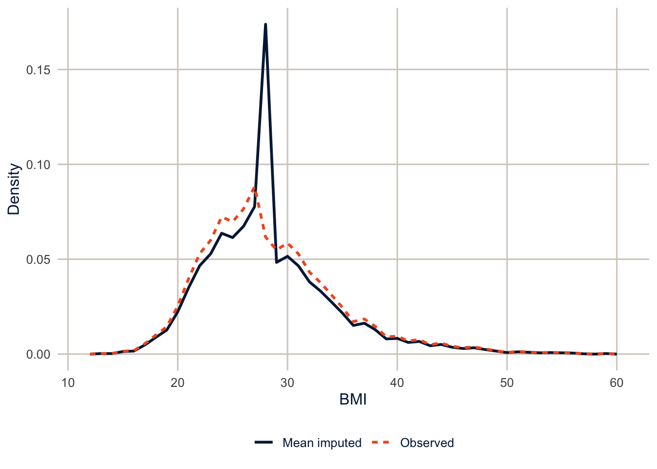
Modal imputation
For a categorical variable, the equivalent is to fill in the most common category. Do that with income, and everyone who didn’t report an income gets put in the most common income group, which changes the whole distribution.
mode_income <- names(which.max(table(tx$income)))
income_mode_imp <- replace_na(as.character(tx$income), mode_income)

tibble(income = levels(tx$income)) |>
  mutate(observed = as.numeric(prop.table(table(tx$income))),
         mode_imputed = as.numeric(prop.table(table(factor(income_mode_imp, levels = income))))) |>
knitr::kable(digits = 3)| income | observed | mode_imputed |
|---|---|---|
| Under $25k | 0.130 | 0.103 |
| $25k-$50k | 0.225 | 0.179 |
| $50k-$100k | 0.271 | 0.216 |
| $100k+ | 0.373 | 0.502 |
NoteCode explanation: finding the mode
table(tx$income) counts each income group. which.max() returns the position of the largest count (with its name attached), and names() pulls out the name, so mode_income is the label of the most common group. replace_na() fills each missing value with it.
Regression imputation, hot deck and predictive mean matching
Better ideas use what we know about the person.
- Regression imputation fits a model for the variable with missing values, using the complete cases, and plugs in each missing person’s predicted value. It uses the relationships in the data, but everyone with the same predictors gets the same imputed value, so it still understates the variance.
- Hot deck imputation finds respondents who look like the person with the missing value on the variables that are observed (the “donors”) and borrows a donor’s actual answer. The Census Bureau did this for decades, and the ACS still does.
- Predictive mean matching (PMM) combines the two. Fit the regression, compute predicted values for everyone, then for each missing case, find a few observed cases whose predicted values are close to the missing case’s, and borrow one of their actual values at random. Because the imputed values are real observed values, they’re always plausible (no negative BMIs, no income category 3.6), and the randomness keeps the variance honest.
Any of these fills in each missing value once, and then we analyze the data as if the imputed values were real. That’s the remaining problem: we don’t know the missing values, and a single imputation hides that uncertainty. The analysis treats a guess as if it had been observed, so its standard errors only reflect sampling, not our uncertainty about what the missing values were. You’ll see exactly how much that understates the standard errors at the end of the chapter.
Investigating patterns of missingness
Flag variables
Before imputing, look at who’s missing. Make a flag that’s 1 if a value is missing, and model it with the things you observe.
flag_fit <- glm(is.na(income_n) ~ badhealth + educ + agec + female + race_eth,
                family = binomial, data = tx)

broom::tidy(flag_fit) |>
  select(term, estimate, std.error, p.value) |>
knitr::kable(digits = 3)| term | estimate | std.error | p.value |
|---|---|---|---|
| (Intercept) | -0.830 | 0.156 | 0.000 |
| badhealth | -0.022 | 0.078 | 0.782 |
| educHS graduate | -0.235 | 0.127 | 0.065 |
| educSome college | -0.484 | 0.128 | 0.000 |
| educCollege graduate | -0.424 | 0.124 | 0.001 |
| agec25-34 | -0.746 | 0.126 | 0.000 |
| agec35-44 | -0.475 | 0.120 | 0.000 |
| agec45-54 | -0.415 | 0.122 | 0.001 |
| agec55-64 | -0.464 | 0.124 | 0.000 |
| agec65+ | 0.025 | 0.109 | 0.818 |
| female | 0.155 | 0.060 | 0.010 |
| race_ethNH Black | -0.135 | 0.106 | 0.203 |
| race_ethNH Other | 0.448 | 0.118 | 0.000 |
| race_ethNH Multiracial | 0.073 | 0.198 | 0.713 |
| race_ethHispanic | -0.023 | 0.081 | 0.775 |
is.na(income_n) is TRUE (1) when income is missing, so this is an ordinary logit model (glm() without the design, since we’re only looking for patterns) of the probability that income is missing.
Missing income is clearly related to education, age and sex (and, for the NH Other group, race and ethnicity), so income is not MCAR, and complete-case analysis would keep a sample that’s more educated and differs in age from the full one. Interestingly, once those are in the model, reporting income isn’t related to self-rated health.
Warning
This is easy to get wrong, so I want to be careful. A test like this can show that data are not MCAR. It can never show that they are MAR, because MAR is about whether missingness depends on the missing values themselves, and those are exactly the values you don’t have. A flag model with no significant predictors tells you the missingness isn’t related to what you observed, and that’s all. Whether income is MAR or MNAR is a judgment about how people answer surveys, and you defend it with substantive arguments and sensitivity analyses, not with a p-value.
Multiple imputation
The idea
Multiple imputation, due to Rubin (1987), deals with the uncertainty problem directly. It doesn’t reveal the missing values. Instead, it creates several plausible completed data sets under stated assumptions, and the differences between their results represent our uncertainty about what was missing. Fill in each missing value \(m\) times, each time with a random draw from a model of what the value might be. That gives \(m\) complete data sets that agree on the observed values and differ on the imputed ones. Analyze each one the way you would have analyzed the complete data, and combine the results.
In words, the combining rules say: the estimate is the average of the \(m\) estimates, and the uncertainty has two parts. One is the ordinary uncertainty you’d have if the data were complete (the average of the \(m\) squared standard errors). The other is how much the \(m\) estimates disagree with each other, which is the uncertainty that comes from not knowing the missing values. Add the two, and that’s the total. Formally, these are Rubin’s rules:
- The combined estimate is the average of the \(m\) estimates, \(\bar Q = \frac{1}{m}\sum_{i=1}^m \hat Q_i\).
- The within-imputation variance \(\bar W\) is the average of the \(m\) squared standard errors, the uncertainty we’d have if the data were complete.
- The between-imputation variance \(B = \frac{1}{m-1}\sum_{i=1}^m (\hat Q_i - \bar Q)^2\) measures how much the estimates disagree because of the missing data.
- The total variance is \(T = \bar W + (1 + \frac{1}{m})B\), and the standard error is \(\sqrt{T}\).
The fraction of missing information (FMI) is roughly \((1 + 1/m)B / T\), the share of the total variance that’s due to the missing data. It’s often much smaller than the share of cases with a missing value, because the other variables carry a lot of information about the missing ones.
Chained equations
With several variables missing in different combinations, mice uses multiple imputation by chained equations (Buuren 2018). It starts by filling every missing value with a random draw from the observed values. Then it goes through the variables one at a time, fitting a model for each one using all the others, and replacing that variable’s missing values with draws from the model. One pass through all the variables is an iteration. After a number of iterations, the imputations settle down, and the last one becomes one imputed data set. The whole thing runs \(m\) times.
Patterns of missingness
md.pattern() shows which combinations of variables are missing together.
patterns <- md.pattern(select(tx, all_of(analysis_vars)), plot = FALSE)
head(patterns, 8)
#> badhealth agec female educ_n race_eth insured smoke bmi income_n
#> 5099 1 1 1 1 1 1 1 1 1 0
#> 821 1 1 1 1 1 1 1 1 0 1
#> 262 1 1 1 1 1 1 1 0 1 1
#> 185 1 1 1 1 1 1 1 0 0 2
#> 203 1 1 1 1 1 1 0 1 1 1
#> 57 1 1 1 1 1 1 0 1 0 2
#> 77 1 1 1 1 1 1 0 0 1 2
#> 236 1 1 1 1 1 1 0 0 0 3tail(patterns, 1)#> badhealth agec female educ_n race_eth insured smoke bmi income_n
#> 0 0 0 51 209 370 640 895 1538 3703Each row is a pattern, with 1 for observed and 0 for missing. The row names are how many respondents have that pattern, the last column is how many variables they’re missing, and the last row (from tail()) is the total number missing for each variable. The first row is the complete cases. Most of the rest are missing just one thing, usually income or BMI. (md.pattern() also draws this as a picture if you leave out plot = FALSE.)
Building the imputation model with a survey design
Two rules matter here, and the second one is where survey data are different.
- Include the outcome. It feels like cheating, but leaving the outcome out of the imputation model imputes values that are unrelated to the outcome, which biases the coefficients toward zero.
- Include the design. The probability of being sampled is related to who people are, and the weights and strata carry that information. Reiter et al. (2006) showed that leaving the design out of the imputation model can bias the results, and that including the design variables (or functions of them) reduces that bias. It doesn’t guarantee unbiased results: the imputation model still has to capture the relationships that matter, like how income relates to education and health. I’ll include the log of the weight and the metro area. Using metro area in place of the strata is an approximation, and one you should justify, not take for granted. Here the justification is that the BRFSS strata are nested within metro areas, so metro area captures the biggest differences between strata, and the 51 Texas strata as a factor would make every imputation model enormous and slow. If the strata within a metro differed a lot in income, this shortcut would miss that.
The first rule deserves a word, because it seems to contradict what you’ll learn about prediction in week 15. There, using the outcome to build a predictor is “leakage,” because the outcome won’t be available when you make a real prediction. Here, we aren’t predicting anything for new people. We’re filling in values in data where the outcome is already observed, so that the analysis of these data is unbiased. Different goals, different rules.
There’s one more choice. Income and education are ordered categories. If I leave them as factors, mice uses multinomial logit models to impute them, which ignore the ordering and are slow. As integer codes with PMM, the imputed values are always one of the observed categories, and the ordering is used. Be clear about what that buys. Because PMM borrows a real, observed category, every imputed value is a possible one. But the matching step uses a linear regression on the 1, 2, 3, … codes, which treats the categories as equally spaced, the same assumption you were warned about in week 5. That’s a reasonable approximation for finding similar people, not a claim that the codes are real numbers, and the analysis model below still treats income and education as categories (factor()).
imp_data <- tx |>
  select(all_of(analysis_vars), place, log_wt)

ini <- mice(imp_data, maxit = 0)
ini$method
#> badhealth income_n educ_n race_eth agec female smoke bmi
#> "" "pmm" "pmm" "polyreg" "" "" "polyreg" "pmm"
#> insured place log_wt
#> "pmm" "" ""
NoteCode explanation:
mice() with maxit = 0
Running mice() with zero iterations doesn’t impute anything, but it sets everything up and tells you what it would do. ini$method shows the imputation method for each variable: "pmm" for numeric ones, "logreg" for two-category factors, "polyreg" (multinomial logit) for unordered factors with more than two categories, and "" for variables with nothing missing. If you want to change a method, or stop a variable from being used to predict others, you edit ini$method or ini$predictorMatrix and pass them back to mice(). Here the defaults are what I want.
How many imputations?
The old advice was that 5 imputations are enough, and for the point estimates, it usually is. For standard errors that don’t change when you rerun the imputation with a new seed, you need more. von Hippel (2020) gives a two-stage rule. Run a small pilot, estimate the largest fraction of missing information, and then use
\[m = 1 + \frac{1}{2}\left(\frac{FMI}{CV}\right)^2\]
where \(CV\) is how much you’re willing to let the standard errors vary from one run to the next (0.05 means 5%). I’ll write a function that analyzes a set of imputations with the design, since we’ll use it twice.
f_health <- badhealth ~ factor(income_n) + factor(educ_n) + race_eth + agec +
  female + smoke + bmi + insured

analyze_mi <- function(imp) {
  completed <- complete(imp, action = "all") |>
    map(\(d) mutate(d, ststr = tx$ststr, mmsawt = tx$mmsawt))
  des_mi <- svydesign(ids = ~1, strata = ~ststr, weights = ~mmsawt,
                      data = imputationList(completed))
  fits <- with(des_mi, svyglm(f_health, family = quasibinomial))
  MIcombine(fits)
}
NoteCode explanation: analyzing imputed survey data
complete(imp, action = "all")returns a list of the \(m\) completed data sets.map(\(d) mutate(d, ...))adds the strata and weights back to each one. I left them out of the imputation data, and since nothing in them is missing, they’re the same in every data set.imputationList()tellssvydesign()that its data are a set of imputations. The result is a list of \(m\) survey designs, all with the same strata and weights.with(des_mi, svyglm(...))fits the same model to each design, giving \(m\) fitted models.MIcombine()applies Rubin’s rules and returns the combined coefficients, the combined variance matrix and the fraction of missing information for each coefficient ($missinfo).
This keeps the survey design in every step. The usual mice workflow, with(imp, glm(...)) and pool(), would ignore it.
pilot <- mice(imp_data, m = 5, maxit = 10, seed = 7283, printFlag = FALSE)
pilot_fit <- analyze_mi(pilot)
max_fmi <- max(pilot_fit$missinfo)
m_needed <- ceiling(1 + 0.5 * (max_fmi / 0.05)^2)
c(max_fmi = max_fmi, m_needed = m_needed)
#> max_fmi m_needed
#> 0.2482943 14.0000000The largest fraction of missing information in the pilot is 0.25, and the rule says we need about 14 imputations for standard errors stable to within 5%. I’ll use 20, which is comfortably more. (von Hippel (2020) suggests using the upper end of a confidence interval for the FMI, which is a bit more conservative.)
imp <- mice(imp_data, m = 20, maxit = 10, seed = 7283, printFlag = FALSE)
mi_fit <- analyze_mi(imp)
This takes a few minutes, and the chunk is cached, so it only runs again if the code changes.
Checking the imputations
Before using the results, check two things. First, did the chained equations settle down? Each line below is one imputation’s mean of the imputed BMI values at each iteration. If they mix together and don’t trend up or down, the algorithm has converged.
tibble(iteration = rep(1:10, times = 20),
       imputation = rep(1:20, each = 10),
       mean_bmi = as.vector(imp$chainMean["bmi", , ])) |>
  ggplot(aes(x = iteration, y = mean_bmi, group = imputation)) +
  geom_line(colour = utsa_cols("midnight"), alpha = 0.5) +
  scale_x_continuous(breaks = 1:10) +
  labs(x = "Iteration", y = "Mean of imputed BMI")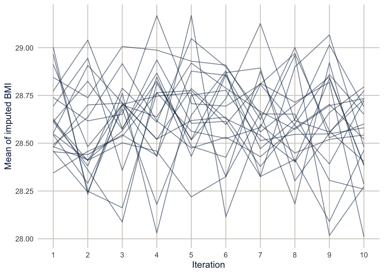
Second, do the imputed values look plausible? They don’t have to match the observed values (if the data are MAR and not MCAR, they shouldn’t), but they should be in the same range.
complete(imp, action = "long") |>
  mutate(imputed = rep(is.na(imp_data$bmi), times = 20)) |>
  filter(imputed | .imp == 1, bmi < 60) |>
  mutate(source = if_else(imputed, "Imputed", "Observed")) |>
  ggplot(aes(x = bmi, colour = source, linetype = source)) +
  geom_density(linewidth = 1) +
  scale_colour_utsa(palette = "primary") +
  labs(x = "BMI", y = "Density", colour = NULL, linetype = NULL)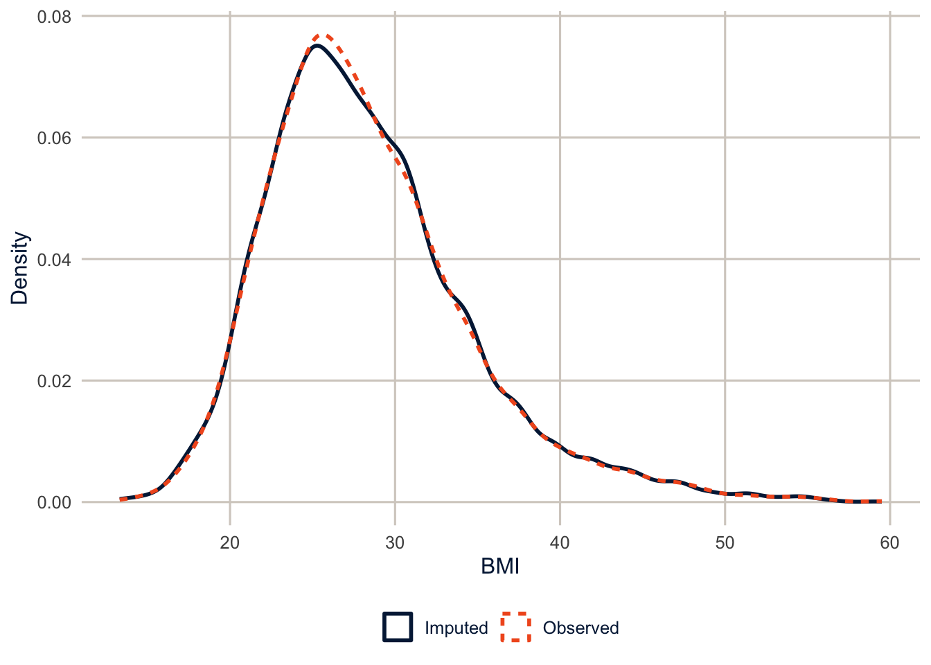
NoteCode explanation: the diagnostic plots
imp$chainMeanis an array with one row per variable, one column per iteration and one layer per imputation, holding the mean of the imputed values.as.vector()flattens the BMI slice column by column, which is why theiterationandimputationvectors are built withrep(..., times = )andrep(..., each = ).complete(imp, action = "long")stacks all 20 completed data sets into one long data frame, with.impsaying which imputation each row came from. To separate the observed values from the imputed ones, I flag the rows where BMI was missing in the original data, repeated 20 times, and keep the observed values only once (.imp == 1).micehas its own plots (plot(imp),densityplot(imp),stripplot(imp)), which are quicker to type but use thelatticepackage and its colors.
The imputed BMI values have almost the same distribution as the observed ones (a mean of 28.51, against 28.49), and none of them are implausible, which is what PMM guarantees. They don’t have to agree this closely. Here, the people missing BMI aren’t very different from everyone else on the things that predict BMI.
Comparing complete cases and multiple imputation
des <- svydesign(ids = ~1, strata = ~ststr, weights = ~mmsawt, data = tx)
fit_cc <- svyglm(f_health, design = des, family = quasibinomial)

compare <- tibble(term = names(coef(fit_cc)),
                  complete_case = coef(fit_cc),
                  se_complete_case = SE(fit_cc),
                  multiple_imputation = coef(mi_fit),
                  se_multiple_imputation = sqrt(diag(vcov(mi_fit))),
                  fmi = mi_fit$missinfo)
knitr::kable(compare, digits = 3)| term | complete_case | se_complete_case | multiple_imputation | se_multiple_imputation | fmi |
|---|---|---|---|---|---|
| (Intercept) | -2.084 | 0.468 | -2.059 | 0.372 | 0.049 |
| factor(income_n)2 | -0.775 | 0.195 | -0.578 | 0.177 | 0.197 |
| factor(income_n)3 | -1.063 | 0.207 | -0.976 | 0.200 | 0.217 |
| factor(income_n)4 | -1.471 | 0.226 | -1.382 | 0.217 | 0.184 |
| factor(educ_n)2 | -0.004 | 0.237 | -0.354 | 0.192 | 0.036 |
| factor(educ_n)3 | -0.089 | 0.231 | -0.405 | 0.192 | 0.033 |
| factor(educ_n)4 | -0.569 | 0.240 | -0.816 | 0.208 | 0.041 |
| race_ethNH Black | -0.111 | 0.215 | -0.131 | 0.178 | 0.050 |
| race_ethNH Other | 0.084 | 0.327 | 0.141 | 0.240 | 0.034 |
| race_ethNH Multiracial | -0.009 | 0.365 | 0.167 | 0.295 | 0.034 |
| race_ethHispanic | 0.387 | 0.172 | 0.311 | 0.144 | 0.044 |
| agec25-34 | -0.593 | 0.290 | -0.500 | 0.231 | 0.017 |
| agec35-44 | -0.104 | 0.300 | -0.033 | 0.236 | 0.022 |
| agec45-54 | 0.253 | 0.297 | 0.460 | 0.230 | 0.029 |
| agec55-64 | 0.694 | 0.279 | 0.720 | 0.221 | 0.017 |
| agec65+ | 0.493 | 0.273 | 0.639 | 0.216 | 0.024 |
| female | 0.093 | 0.138 | 0.118 | 0.115 | 0.020 |
| smokeFormer | 0.602 | 0.165 | 0.515 | 0.145 | 0.102 |
| smokeCurrent | 0.582 | 0.232 | 0.684 | 0.198 | 0.121 |
| bmi | 0.045 | 0.011 | 0.043 | 0.009 | 0.075 |
| insured | -0.248 | 0.196 | -0.114 | 0.178 | 0.110 |
compare |>
  filter(term != "(Intercept)") |>
  pivot_longer(c(complete_case, multiple_imputation), names_to = "method", values_to = "estimate") |>
  mutate(se = if_else(method == "complete_case", se_complete_case, se_multiple_imputation),
         method = if_else(method == "complete_case", "Complete cases", "Multiple imputation")) |>
  ggplot(aes(x = estimate, y = fct_rev(fct_inorder(term)), colour = method, shape = method)) +
  geom_vline(xintercept = 0, colour = utsa_cols("smoke")) +
  geom_pointrange(aes(xmin = estimate - 1.96 * se, xmax = estimate + 1.96 * se),
                  position = position_dodge(width = 0.6)) +
  scale_colour_utsa(palette = "primary") +
  labs(x = "Log-odds", y = NULL, colour = NULL, shape = NULL)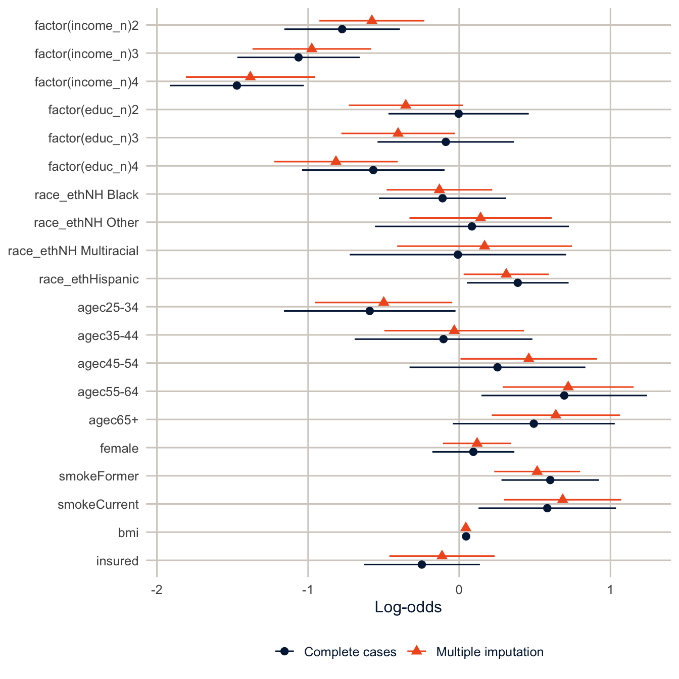
Three things to see here. First, the standard errors from multiple imputation are smaller for nearly every coefficient, because we’re using 7,509 respondents instead of 5,099. Second, some estimates move. With complete cases, high school graduates and people with some college look no different from people without a high school diploma (coefficients of 0 and -0.09), and only college graduates stand out (-0.57). After imputation, all three are clearly negative (-0.35, -0.4 and -0.82). Remember that less educated respondents are less likely to report their income, so complete-case analysis drops them disproportionately, and with them a good part of the education gradient. Third, the FMI column is largest for the income coefficients, up to 0.22, because income is the most-missing variable, but it’s well below the 20% of respondents missing income, because education, age and the rest tell us a lot about income.
TipReading the result: a right and a wrong interpretation
Right: “Assuming income and BMI are missing at random given the variables in the imputation model, college graduates have log-odds of fair or poor health 0.82 lower than adults without a high school diploma, with the same income, race and ethnicity, age, sex, smoking, BMI and insurance. The complete-case estimate is 0.57 lower.”
Wrong: “Multiple imputation recovered the true incomes, so the imputed results are correct.” Imputation doesn’t reveal anything; the imputed results are only as good as the MAR assumption and the imputation model. And if the complete-case and imputed results had agreed, that wouldn’t prove the assumption either; both could be biased in the same way if income is MNAR.
What a single imputation would have said
Here’s the uncertainty problem from earlier, in numbers. Take just one of the imputed data sets and analyze it as if it were complete. That’s what you’d get from any single-imputation method.
des_single <- svydesign(ids = ~1, strata = ~ststr, weights = ~mmsawt,
                        data = mutate(complete(imp, action = 1),
                                      ststr = tx$ststr, mmsawt = tx$mmsawt))
fit_single <- svyglm(f_health, design = des_single, family = quasibinomial)

tibble(term = names(coef(fit_single)),
       se_single_imputation = SE(fit_single),
       se_multiple_imputation = sqrt(diag(vcov(mi_fit)))) |>
  mutate(ratio = se_multiple_imputation / se_single_imputation) |>
  filter(str_detect(term, "income")) |>
knitr::kable(digits = 3)| term | se_single_imputation | se_multiple_imputation | ratio |
|---|---|---|---|
| factor(income_n)2 | 0.159 | 0.177 | 1.115 |
| factor(income_n)3 | 0.183 | 0.200 | 1.091 |
| factor(income_n)4 | 0.197 | 0.217 | 1.103 |
complete(imp, action = 1) pulls out just the first completed data set. For the income coefficients, where the missing information is greatest, the single-imputation standard errors are smaller than the multiple-imputation ones. The single imputation treats every imputed income as if it had been observed, so it leaves out the between-imputation part of Rubin’s rules, and its standard errors are too small.
Tip
Multiple imputation doesn’t create information. It uses the information in the observed variables about the missing ones, and it’s honest about what’s left over. If your imputation model is wrong (it leaves out an interaction the analysis model includes, for example), the imputations will be wrong in the same way. The rule of thumb is that the imputation model should be at least as rich as the analysis model, and include anything that predicts the missing values or whether they’re missing.
Summary
Complete-case analysis is the default everywhere. It’s guaranteed to be unbiased only when the data are MCAR, which they almost never are, and whether it’s biased otherwise depends on what you’re estimating and why the data are missing. Mean and modal imputation keep the sample size but distort distributions and shrink variances, so don’t use them. Multiple imputation fills in the missing values several times, analyzes each completed data set, and combines the results with Rubin’s rules, so the standard errors include the uncertainty from the missing data. With survey data, put the design variables in the imputation model and analyze each imputed data set with the design, using imputationList() and MIcombine(). You can show that data aren’t MCAR, but you can never show from the data that they’re MAR, so you have to argue for it. For more, Allison (2002) is a short and readable introduction, Schafer and Graham (2002) is a classic review, and Buuren (2018) covers mice in detail and is free online.
Homework 9
Due: March 25, before class.
Which version to do. If you’re in DEM 7283, do the version with your own survey data. If you’re in DEM 5283, do either version, and say at the top of your homework which one you did. If your survey can’t support this week’s method, do the version with my data and say so.
Purpose. Reason about why data are missing, impute them in a way that keeps the survey design, and be honest about what the imputation assumes.
A satisfactory answer states the missingness assumption behind each analysis; reports estimates with standard errors or confidence intervals; and doesn’t claim that a test, or agreement between two analyses, proves that the data are MAR.
With your own survey data
Use the full survey design for every estimate unless a step says otherwise, and report each estimate with a standard error or confidence interval.
- Use your survey data.
- Measure an outcome variable and at least five predictors.
- Report the pattern of missingness among all of these variables.
- What share of cases would a complete-case analysis drop?
- Make a flag for missingness on the variable with the most missing data, and model the flag with the other variables. Is that variable MCAR? Who is less likely to answer it?
- Describe one plausible reason for the missing data that would make it MAR, and one that would make it MNAR.
- Perform a mean imputation for numeric data or a modal imputation for categorical data for all missing values.
- Perform the analysis using the imputed data and the survey design.
- What are your results?
- Perform a multiple imputation of all missing values with
mice(), including the design variables (weight, strata and PSU) in the imputation model.- Check the convergence of the imputations.
- Perform the analysis on each imputed dataset with the survey design, and combine the results with Rubin’s rules.
- What are your results?
- Compare the approaches:
- Were the results similar between the mean/modal-imputed and multiply imputed datasets? Compare the standard errors as well as the estimates.
- How do these results compare with the complete-case model fit using the original data with missing values?
- Explain why agreement (or disagreement) between the analyses doesn’t prove that the data are MAR.
With my data
What is provided. The Texas BRFSS data tx, the imputation data imp_data, the analysis formula f_health, the function analyze_mi(), and the 20 imputations in imp from this chapter.
1. Describe one plausible explanation for missing income that would make it MAR, and one that would make it MNAR, using what you know about how people answer surveys. Then compare the complete-case and multiple-imputation estimates of the income coefficients from this chapter, including their standard errors. Explain in two or three sentences why agreement (or disagreement) between the two doesn’t prove that the missingness assumption is correct.
2. Make a flag for missing BMI and model it with the same predictors as the income flag model. Is BMI MCAR? Who is less likely to report their height and weight?
# YOUR CODE HERE3. Rerun the final imputation with m = 5 and a different seed, and compare the standard errors of the income coefficients to the ones from m = 20. How much do they change? Relate your answer to the von Hippel rule.
# YOUR CODE HERE4. Rerun the imputation without place and log_wt in the imputation model, analyze it with the design, and compare the coefficients to the ones above. Do any of them move by more than a standard error?
# YOUR CODE HEREOne solution for exercise 4
imp_nodesign <- mice(select(imp_data, -place, -log_wt), m = 20, maxit = 10,
                     seed = 7283, printFlag = FALSE)
fit_nodesign <- analyze_mi(imp_nodesign)

tibble(term = names(coef(mi_fit)),
       with_design = coef(mi_fit),
       without_design = coef(fit_nodesign),
       difference_in_se = (without_design - with_design) / sqrt(diag(vcov(mi_fit)))) |>
  knitr::kable(digits = 3)
analyze_mi() still uses the design for the analysis, which is what you want. Only the imputation model changes.
5. Using the imputed data, estimate the prevalence of fair or poor health by income group with svyby(), and compare it to the complete-case estimate. (Hint: with(des_mi, svyby(...)) returns one result per imputation; MIcombine() combines them. You’ll need to rebuild des_mi outside the function.)
# YOUR CODE HEREOne solution for exercise 5
completed <- complete(imp, action = "all") |>
  map(\(d) mutate(d, ststr = tx$ststr, mmsawt = tx$mmsawt))
des_mi <- svydesign(ids = ~1, strata = ~ststr, weights = ~mmsawt,
                    data = imputationList(completed))

prev_mi <- with(des_mi, svyby(~badhealth, ~income_n, design = .design, FUN = svymean)) |>
  MIcombine()
prev_mi

svyby(~badhealth, ~income_n, design = des, FUN = svymean, na.rm = TRUE)
Inside with() on an imputation list, the current design is called .design.
6. A sensitivity analysis for MNAR. Suppose people who didn’t report their income actually earn less than MAR-based imputation predicts: one income category lower, on average. Rerun the imputation with every imputed income moved down one category (but not below the lowest), analyze it with analyze_mi(), and compare the education and income coefficients with the ones above. How much would this kind of MNAR change your conclusions?
# YOUR CODE HEREA hint for exercise 6
mice() can change each imputed value right after it’s drawn, with the post argument. Start from ini <- mice(imp_data, maxit = 0), then set post <- ini$post and post["income_n"] <- "imp[[j]][, i] <- pmax(1, imp[[j]][, i] - 1)", and pass post = post to mice(). pmax(1, x - 1) subtracts 1 but never goes below 1. This is called a delta adjustment, and you can try shifts of different sizes to see how big an MNAR problem would have to be to change your conclusions.
Additional resources
- Flexible Imputation of Missing Data (Buuren 2018), free online, by the author of
mice. If you read one thing on multiple imputation, read this. - Allison (2002), Missing Data, is a short Sage book and a very good first read on why complete-case analysis fails and what the alternatives assume.
- The
micewebsite has a series of hands-on vignettes, from a first imputation to diagnostics and passive imputation. - von Hippel (2020) on how many imputations you need, which is the rule this chapter uses.