Week 10: Longitudinal Models

Introduction

Everything so far has used cross-sectional data: each person is observed once. Longitudinal (or panel) data follow the same people over time, and that changes two things. First, observations on the same person are correlated, so the independence assumption behind every model so far is wrong, and the standard errors will be too. Second, and more interesting, we can compare a person to themselves at different times, which lets us hold constant everything about them that doesn’t change, whether we measured it or not.

This week covers both. Generalized estimating equations (GEEs) handle the correlation and give population-average effects. Fixed effects models use only the changes within each person. Random effects models do something in between, and the within-between model shows you exactly what that “something” is, by estimating the within-person and between-person effects separately. The example is children’s math scores and family poverty from kindergarten through fifth grade.

Here’s the distinction that runs through the whole chapter, with three made-up children followed for three years:

Child	Year 1	Year 2	Year 3	Average score
Ana (never poor)	50	60	70	60
Ben (always poor)	30	40	50	40
Cal (poor in year 2 only)	45	55 (poor)	65	55

There are two different questions here. Between children: do children in poorer families score lower than other children? Yes: Ben, who is always poor, averages 20 points below Ana. Within a child: does a child’s score change when that child’s family becomes poorer? Look at Cal. His scores rise by 10 points a year whether or not his family is poor, so his poor year isn’t lower than his own trend. These two comparisons use different information (differences between children, and changes within a child), and they need not have the same answer. Here they don’t.

NoteThis week at a glance

The question. Do children in poor families score lower in math, and do a child’s scores change when their own family’s poverty status changes?

By the end of this week you should be able to

1. reshape repeated measurements from wide to long format, and explain why the number of rows isn’t the number of independent people;
2. explain the difference between a between-child and a within-child comparison, and say which variation each model uses;
3. fit GEE, fixed effects and within-between models, interpret the within and between terms in score units, and say what a fixed effects model does and doesn’t control for.

Before you begin. You need linear regression, pivot_longer() and pivot_wider() (from week 7), and clustered standard errors from week 2.

Required and optional. The estimating equation for GEE is there for reference; the “cookbook version” is what you need.

Setup

geepack fits GEEs (Højsgaard et al. 2006), fixest fits fixed effects models quickly (Berg’e et al. 2026), and lme4 fits random effects models (Bates et al. 2015), which we’ll use much more in weeks 12 and 13.

library(tidyverse)
library(here)
library(geepack)
library(fixest)
library(lme4)
library(modelsummary)
library(sparkscolors)  # pak::pak("coreysparks/sparkscolors"), UTSA colors

The data: ECLS-K:2011

The Early Childhood Longitudinal Study, Kindergarten Class of 2010-11 (National Center for Education Statistics 2019) followed a nationally representative sample of children from kindergarten through fifth grade, testing them in math and reading and interviewing their parents at nine rounds. The full public-use file has 18,174 children and over 26,000 variables, so I made a smaller file with the variables we need (the script is R/make_eclsk_subset.R).

I’ll use the six spring rounds where the parent interview measured family poverty: spring of kindergarten (round 2), first grade (4), second grade (6), third grade (7), fourth grade (8) and fifth grade (9). The weight is the K-5 longitudinal weight, w9c29p_9a0, which is positive only for children who took part in every round. Applying it means the analysis describes the population of children who were in kindergarten in 2010-11, adjusted for the design and for attrition (children dropping out of the study over the years), as far as the adjustment can go. It corrects for attrition related to the characteristics the weighting used, not for every reason a child might have left, and it doesn’t do anything about the scattered items (a missing test score in one round, say) that we drop below. Those are week 9’s problem.

ECLS-K codes missing values as negative numbers (-1 for not applicable, -7 for refused, -8 for don’t know, -9 for not ascertained), so the first step is to turn those into NA.

Time-constant and time-varying variables

Panel data have two kinds of variables. Time-constant (or time-invariant) variables have one value per child: sex, race and ethnicity, the design variables. Time-varying variables are measured at each round: the test scores, age, and poverty. In the file, the time-varying ones have one column per round, with the round number in the name, like x2mscalk5 and x4mscalk5 for the math scores in rounds 2 and 4. That’s wide format.

neg_to_na <- function(x) if_else(x < 0, NA_real_, as.numeric(x))

eclsk_wide <- readRDS(here("data", "eclsk2011_k5.rds")) |>
  filter(w9c29p_9a0 > 0) |>
  transmute(childid,
            # time-constant
            wt = w9c29p_9a0,
            stratum = w9c29p_9astr,
            psu = paste(w9c29p_9astr, w9c29p_9apsu),
            female = if_else(x_chsex_r == 2, 1, 0),
            race = factor(case_when(x_raceth_r == 1 ~ "White",
                                    x_raceth_r == 2 ~ "Black",
                                    x_raceth_r %in% 3:4 ~ "Hispanic",
                                    x_raceth_r == 5 ~ "Asian",
                                    x_raceth_r > 5 ~ "Other"),
                          levels = c("White", "Black", "Hispanic", "Asian", "Other")),
            # time-varying: math score, age in years, family below the poverty line
            math_2 = neg_to_na(x2mscalk5), math_4 = neg_to_na(x4mscalk5),
            math_6 = neg_to_na(x6mscalk5), math_7 = neg_to_na(x7mscalk5),
            math_8 = neg_to_na(x8mscalk5), math_9 = neg_to_na(x9mscalk5),
            age_2 = neg_to_na(x2kage_r) / 12, age_4 = neg_to_na(x4age) / 12,
            age_6 = neg_to_na(x6age) / 12, age_7 = neg_to_na(x7age) / 12,
            age_8 = neg_to_na(x8age) / 12, age_9 = neg_to_na(x9age) / 12,
            poor_2 = as.numeric(neg_to_na(x2povty) == 1),
            poor_4 = as.numeric(neg_to_na(x4povty_i) == 1),
            poor_6 = as.numeric(neg_to_na(x6povty_i) == 1),
            poor_7 = as.numeric(neg_to_na(x7povty_i) == 1),
            poor_8 = as.numeric(neg_to_na(x8povty_i) == 1),
            poor_9 = as.numeric(neg_to_na(x9povty_i) == 1))

nrow(eclsk_wide)

#> [1] 8542

transmute() is like mutate(), but it keeps only the columns it creates (and any you name, like childid). neg_to_na() is a small function, written on the first line, that turns every negative code into NA. paste(w9c29p_9astr, w9c29p_9apsu) glues the stratum and PSU numbers into one label, so each PSU gets a unique name.

The poverty variables have three categories (below the poverty line, 100-199% of it, and 200% or more), and I’ve made an indicator for being below the line.

Reshaping to long format

Every model this week wants long format: one row per child per round, with one column for each variable. Here’s the difference for two children and two rounds:

Wide: one row per child

childid	female	math_2	math_4	poor_2	poor_4
101	1	45	62	0	0
102	0	38	51	1	0

Long: one row per child per round

childid (person)	round (time)	female	math	poor
101	2	1	45	0
101	4	1	62	0
102	2	0	38	1
102	4	0	51	0

The long version has two identifier columns, the person identifier (childid) and the time variable (round), and each time-varying variable becomes one column. Time-constant variables like female repeat on every row for that child. pivot_longer() does the reshaping.

eclsk <- eclsk_wide |>
  pivot_longer(cols = matches("_[0-9]$"),
               names_to = c(".value", "round"),
               names_sep = "_") |>
  mutate(round = as.integer(round)) |>
  filter(!is.na(math), !is.na(age), !is.na(poor), !is.na(race)) |>
  arrange(childid, round)

eclsk |>
  select(childid, round, age, math, poor, female, race) |>
  head(8) |>
  knitr::kable(digits = 2)

childid	round	age	math	poor	female	race
10000001	2	6.65	70.76	0	0	White
10000001	4	7.64	93.21	0	0	White
10000001	6	8.64	111.03	0	0	White
10000001	7	9.59	122.10	0	0	White
10000001	8	10.59	132.78	1	0	White
10000001	9	11.59	135.76	0	0	White
10000006	2	6.89	33.75	0	1	White
10000006	4	7.90	51.27	0	1	White

NoteCode explanation: pivot_longer() with .value

1. cols = matches("_[0-9]$") picks the columns whose names end in an underscore and a digit: all the time-varying ones. The time-constant columns stay as they are and get repeated on every row for that child.
2. names_sep = "_" splits each name at the underscore, so math_4 becomes "math" and "4".
3. names_to = c(".value", "round") says what to do with the two pieces. ".value" is a special name that means “the first piece is the name of the new column the value goes in,” so all the math_ columns become one math column, all the age_ columns become one age column, and so on. The second piece goes in a new column called round.

This is why I named the time-varying variables name_round. A consistent naming scheme turns a messy reshape into one function call.

That leaves 48,149 child-rounds for 8,514 children. Notice those are very different numbers. The rows aren’t 48,149 independent observations, because each child contributes up to six of them, and a child’s scores in different rounds are related. Here is what math growth looks like for the first ten children.

first10 <- unique(eclsk$childid)[1:10]

eclsk |>
  filter(childid %in% first10) |>
  ggplot(aes(x = age, y = math, group = childid)) +
  geom_line(colour = utsa_cols("midnight"), alpha = 0.6) +
  geom_point(colour = utsa_cols("midnight"), size = 1) +
  labs(x = "Age (years)", y = "Math scale score")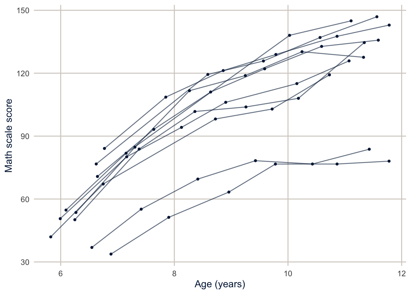

Figure 10.1: Math scores across rounds for ten ECLS-K:2011 children.

Every child’s scores go up, but they start in different places and grow at different rates. Children who start high tend to stay high, and that’s the correlation we need to deal with.

Why ordinary regression gets this wrong

Fit an ordinary regression, ignoring that each child appears up to six times, and look at the correlation between a child’s residuals in different rounds.

fit_ols <- lm(math ~ factor(round) + poor + female + race, data = eclsk, weights = wt)

resid_cor <- eclsk |>
  mutate(resid = residuals(fit_ols)) |>
  select(childid, round, resid) |>
  pivot_wider(names_from = round, values_from = resid, names_prefix = "round_") |>
  select(-childid) |>
  cor(use = "pairwise.complete.obs")

round(resid_cor, 2)

#>         round_2 round_4 round_6 round_7 round_8 round_9
#> round_2    1.00    0.78    0.71    0.66    0.64    0.63
#> round_4    0.78    1.00    0.82    0.76    0.74    0.72
#> round_6    0.71    0.82    1.00    0.84    0.81    0.79
#> round_7    0.66    0.76    0.84    1.00    0.86    0.83
#> round_8    0.64    0.74    0.81    0.86    1.00    0.87
#> round_9    0.63    0.72    0.79    0.83    0.87    1.00

residuals(fit_ols) gives each row’s residual. The pivot_wider() puts each child’s residuals side by side, one column per round, and cor(use = "pairwise.complete.obs") computes the correlation between every pair of rounds, using every child who has both. (lower.tri(), in the text below, picks out the correlations below the diagonal, leaving out the 1s.)

If the observations were independent, these would all be near zero. They’re between 0.63 and 0.87, and they get smaller as the rounds get further apart. A child who does better than the model predicts in kindergarten keeps doing better. Ignoring that does two things to the standard errors. For time-constant predictors like race, each child counts as six observations when they’re really closer to one, so the standard errors are too small. For time-varying predictors, the comparison is partly within children, and the correlation actually helps, so ordinary regression can overstate the standard errors.

Generalized estimating equations

The model

GEEs, introduced by Liang and Zeger (1986), are regression models for the mean response, treating the correlation within a person (or cluster) as a nuisance. They don’t specify a full probability distribution for the data, only the mean, through a link function, and a “working” guess at how the observations on the same person are correlated. They aren’t fit by maximum likelihood. Instead, they solve the estimating equations

\[U(\beta) = \sum_{i=1}^n D_i' V_i^{-1}(y_i - \mu_i(\beta)) = 0\]

where \(y_i\) is the vector of outcomes for person \(i\), \(\mu_i(\beta)\) is the model’s mean for them, \(D_i\) is the derivative of the mean with respect to the coefficients, and \(V_i\) is the working covariance matrix. The cookbook version:

1. Fit an ordinary regression, assuming independence.
2. Compute the residuals and estimate the working correlation among them.
3. Refit the regression, giving correlated observations less weight.
4. Repeat until the coefficients stop changing.

The coefficients are population-average (or marginal) effects: how the mean outcome in the population changes with \(x\). The standard errors are “robust” (sandwich) standard errors, which are valid even if the working correlation is wrong, as long as there are enough people.

Working correlation structures

For three rounds, the four common choices of working correlation are:

Independence, which is ordinary regression: \[\begin{bmatrix} 1 & 0 & 0 \\ 0 & 1 & 0 \\ 0 & 0 & 1 \end{bmatrix}\]

Exchangeable, where every pair of rounds is correlated by the same amount: \[\begin{bmatrix} 1 & \rho & \rho \\ \rho & 1 & \rho \\ \rho & \rho & 1 \end{bmatrix}\]

First-order autoregressive, AR(1), where the correlation shrinks with the distance between rounds: \[\begin{bmatrix} 1 & \rho & \rho^2 \\ \rho & 1 & \rho \\ \rho^2 & \rho & 1 \end{bmatrix}\]

Unstructured, where every pair gets its own correlation: \[\begin{bmatrix} 1 & \rho_1 & \rho_2 \\ \rho_1 & 1 & \rho_3 \\ \rho_2 & \rho_3 & 1 \end{bmatrix}\]

The residual correlations above shrink with distance, which looks like AR(1), but they don’t shrink as fast as \(\rho^2, \rho^3, \ldots\) would, so exchangeable might do as well.

Fitting GEEs

f_math <- math ~ factor(round) + poor + female + race

eclsk <- eclsk |> mutate(w = wt / mean(wt))

gee_ind <- geeglm(f_math, id = childid, waves = round, corstr = "independence",
                  data = eclsk, weights = w)
gee_exch <- geeglm(f_math, id = childid, waves = round, corstr = "exchangeable",
                   data = eclsk, weights = w)
gee_ar1 <- geeglm(f_math, id = childid, waves = round, corstr = "ar1",
                  data = eclsk, weights = w)

modelsummary(list("Independence" = gee_ind, "Exchangeable" = gee_exch, "AR(1)" = gee_ar1),
             coef_omit = "round", gof_map = "nobs", stars = TRUE)

	Independence	Exchangeable	AR(1)
+ p < 0.1, * p < 0.05, ** p < 0.01, *** p < 0.001
(Intercept)	57.352***	56.157***	55.474***
	(0.314)	(0.329)	(0.317)
poor	-8.492***	-1.299***	-0.889***
	(0.445)	(0.213)	(0.205)
female	-2.378***	-2.309***	-1.475***
	(0.362)	(0.376)	(0.357)
raceBlack	-11.590***	-13.625***	-12.701***
	(0.667)	(0.667)	(0.644)
raceHispanic	-6.932***	-9.346***	-8.899***
	(0.453)	(0.436)	(0.416)
raceAsian	3.509***	2.472***	2.115**
	(0.709)	(0.750)	(0.672)
raceOther	-2.330**	-2.986**	-2.907***
	(0.902)	(0.920)	(0.837)
Num.Obs.	48149	48149	48149

NoteCode explanation: geeglm()

1. id = childid says which rows belong to the same cluster (here, the same child). The data must be sorted so that each child’s rows are together, which is why I used arrange(childid, round).
2. waves = round says which round each row is, so the AR(1) structure knows which rounds are adjacent even when a child is missing one.
3. corstr is the working correlation structure.
4. weights = w uses the longitudinal weight, rescaled to average 1 (as in week 7, the scale doesn’t change the estimates, but it keeps the algorithm stable).

The working correlation is 0.79 for the exchangeable model and 0.9 for AR(1). The coefficient for poverty is -8.49 with independence, -1.3 with exchangeable correlation and -0.89 with AR(1). With independence, poverty is mostly a comparison between children, poor and not poor. With a correlation structure, the model weights the observations differently and leans somewhat more on children whose poverty status changes, and the coefficient shrinks. Keep that in mind; it’s the main story of this week.

But don’t read the smaller GEE coefficient as the within-child effect. Every GEE coefficient here is still a population-average comparison that mixes between-child and within-child information, just in different proportions. Changing the working correlation changes the mix; it doesn’t separate the two. If you want the within-child relationship, you have to ask for it directly, which is what fixed effects and the within-between model do.

Choosing a correlation structure

GEEs aren’t fit by maximum likelihood, so there’s no AIC or likelihood ratio test. Pan (2001) proposed the QIC, an information criterion built on the quasi-likelihood, and Hin and Wang (2009) proposed the CIC, which is designed for comparing working correlations with the same mean model. Smaller is better for both.

bind_rows(Independence = QIC(gee_ind), Exchangeable = QIC(gee_exch), `AR(1)` = QIC(gee_ar1),
          .id = "structure") |>
  select(structure, QIC, CIC) |>
  knitr::kable(digits = 1, format.args = list(big.mark = ","))

structure	QIC	CIC
Independence	11,406,836	49.2
Exchangeable	11,819,719	46.4
AR(1)	11,900,317	42.1

QIC() computes the criteria for one model; bind_rows(..., .id = "structure") stacks them with a column of names, as in week 7.

Here the two criteria disagree: QIC prefers the exchangeable structure, and CIC prefers AR(1). That happens, and it’s a reminder that the working correlation is a working assumption. The robust standard errors protect you if it’s wrong, so don’t agonize.

WarningWhat about the survey design?

There are two kinds of clustering in these data, and it’s easy to mix them up. One is the repeated measurements: the rounds for one child are correlated because they’re the same child. The other is the survey design: ECLS-K sampled PSUs (groups of counties) within strata, then schools, then children, so children in the same PSU are correlated with each other too. geeglm() only knows about the first kind. The robust standard errors account for it, but not for the clustering of children within PSUs. The fixest models below can cluster at the PSU level, and that’s the safer choice for published work.

Fixed effects

Comparing children to themselves

Write the model for child \(i\) at round \(t\) with a separate intercept for each child, \(\alpha_i\):

\[y_{it} = \alpha_i + \beta x_{it} + \tau_t + \varepsilon_{it}\]

The \(\alpha_i\) absorb everything about the child that doesn’t change over time: their sex, their race, their parents’ education, the neighborhood they started school in, their genes, their motivation in kindergarten, whether we measured it or not. You can’t estimate the effect of a time-constant variable in this model, because it’s perfectly collinear with the child’s intercept. What’s left is the effect of changes in \(x\) within children. Mechanically, fixed effects estimation subtracts each child’s mean from every variable, \(y_{it} - \bar y_i\) and \(x_{it} - \bar x_i\), and runs regression on what’s left. Allison (2009) is a short, clear introduction.

Notice what that means for poverty. The model splits each child’s poverty into their own average (the share of rounds they were poor) and their deviation from it in each round, and the fixed effects use only the deviations. So in the fixed effects model, the poverty coefficient answers: when a child’s family falls below the poverty line, how does that child’s math score change compared to their own scores in other years? Only the 1,914 children whose poverty status changed at some point contribute to that estimate.

fe <- feols(math ~ poor | childid + round, data = eclsk, weights = ~wt, cluster = ~psu)
ols <- feols(math ~ poor + female + race | round, data = eclsk, weights = ~wt, cluster = ~psu)

etable(ols, fe, headers = c("Pooled OLS", "Child fixed effects"))

#>                                ols                  fe
#>                         Pooled OLS Child fixed effects
#> Dependent Var.:               math                math
#>                                                       
#> poor            -8.492*** (0.4883)    -0.1735 (0.2217)
#> female          -2.378*** (0.3589)                    
#> raceBlack       -11.59*** (0.8608)                    
#> raceHispanic    -6.932*** (0.6157)                    
#> raceAsian        3.509*** (0.8057)                    
#> raceOther         -2.330* (0.9257)                    
#> Fixed-Effects:  ------------------    ----------------
#> round                          Yes                 Yes
#> childid                         No                 Yes
#> _______________ __________________    ________________
#> S.E.: Clustered            by: psu             by: psu
#> Observations                48,149              48,126
#> R2                         0.71937             0.94955
#> Within R2                  0.15766             3.43e-5
#> ---
#> Signif. codes: 0 '***' 0.001 '**' 0.01 '*' 0.05 '.' 0.1 ' ' 1

NoteCode explanation: feols()

1. Everything after the | in the formula is a fixed effect. | childid + round gives every child their own intercept and every round its own intercept, without printing thousands of coefficients. feols() removes them by demeaning, which is why it’s so fast.
2. weights = ~wt uses the longitudinal weight.
3. cluster = ~psu computes standard errors clustered at the PSU, the highest level of the sampling design, which also allows for correlation among the rounds for each child (since every child is inside one PSU). I made psu unique by pasting the stratum and PSU numbers together, because PSU numbers repeat across strata.
4. etable() makes a side-by-side table of fixest models.

The pooled regression says children in poor families score 8.5 points lower in math. The fixed effects model says that when a child’s family becomes poor, their math score changes by -0.17 points, with a standard error of 0.22, which is no detectable change at all. The large gap between poor and non-poor children is almost all a difference between children, not a consequence of a family’s poverty status in a given year.

TipReading the result: a right and a wrong interpretation

Right: “Comparing each child with themselves, math scores in rounds when the child’s family was below the poverty line were -0.17 points different from the child’s scores in other rounds (standard error 0.22), which is no detectable within-child difference.”

Wrong: “Poverty has no effect on children’s math scores.” The fixed effects estimate says nothing about the large difference between children who grow up poor and those who don’t, which is where most of the gap is. It only says that short-run changes in a family’s poverty status aren’t accompanied by changes in that year’s score.

Random effects and the within-between model

Random effects

A random effects model also gives each child their own intercept, but treats the intercepts as draws from a normal distribution, \(\alpha_i \sim N(\alpha, \sigma^2_\alpha)\), instead of estimating each one. (This is the multilevel model of weeks 12 and 13, with rounds nested in children.) It can estimate time-constant effects, and it’s more efficient, but it comes with an assumption: the child intercepts have to be unrelated to the predictors. If poorer families also differ in ways that affect math scores and that we haven’t measured (and they do), that assumption fails, and the random effects coefficient is a mix of the within-child and between-child relationships.

re <- lmer(math ~ factor(round) + poor + female + race + (1 | childid), data = eclsk)
fixef(re)["poor"]

#>      poor 
#> -1.215275

lmer() fits a linear random effects model. (1 | childid) means “a random intercept for each child”; week 12 explains the notation in detail. fixef() pulls out the ordinary (fixed) coefficients.

The random effects estimate, -1.22, sits between the fixed effects estimate and the pooled one. That’s not a coincidence: it’s a weighted average of the within and between relationships.

The within-between model

Mundlak (1978), Allison (2009) and Bell and Jones (2015) suggest a model that keeps the advantages of both. Split the time-varying predictor into two parts: each child’s average over the study, \(\bar x_i\), and their deviation from their own average in each round, \(x_{it} - \bar x_i\). Put both in the model.

\[y_{it} = \beta_0 + \beta_W (x_{it} - \bar x_i) + \beta_B \bar x_i + \gamma z_i + \tau_t + u_i + \varepsilon_{it}\]

\(\beta_W\) is the within effect, and it’s the same as the fixed effects estimate (exactly the same in a balanced panel, and very close in an unbalanced one like this). \(\beta_B\) is the between effect: how children who are poorer on average differ from children who are less poor on average. And because the child intercepts aren’t swept out, the model can still include time-constant variables \(z_i\).

You can fit it as a random effects model with lmer(), which gives you the variance of the child intercepts. But lmer() can’t use survey weights (its weights argument means something else, as we’ll see in week 12), so to compare it with the weighted fixed effects model, I’ll fit the same mean model with feols(), using the weights and clustering the standard errors by PSU.

eclsk <- eclsk |>
  group_by(childid) |>
  mutate(poor_mean = mean(poor),
         poor_within = poor - poor_mean) |>
  ungroup()

wb <- feols(math ~ poor_within + poor_mean + female + race | round,
            data = eclsk, weights = ~wt, cluster = ~psu)

tibble(model = c("Pooled OLS", "Random effects (unweighted)", "Fixed effects",
                 "Within-between: within", "Within-between: between"),
       estimate = c(coef(ols)["poor"], fixef(re)["poor"], coef(fe)["poor"],
                    coef(wb)["poor_within"], coef(wb)["poor_mean"]),
       se = c(se(ols)["poor"], sqrt(vcov(re)["poor", "poor"]), se(fe)["poor"],
              se(wb)["poor_within"], se(wb)["poor_mean"])) |>
  knitr::kable(digits = 2)

model	estimate	se
Pooled OLS	-8.49	0.49
Random effects (unweighted)	-1.22	0.15
Fixed effects	-0.17	0.22
Within-between: within	-0.18	0.22
Within-between: between	-12.15	0.64

NoteCode explanation: group-mean centering

group_by(childid) followed by mutate() computes things within each child. mean(poor) is the share of rounds in which that child’s family was poor, and poor - poor_mean is how far each round is from the child’s own average. ungroup() turns the grouping off so later steps work on the whole data set. You’ll see the same move in week 12, where it’s called group-mean centering.

The within effect, -0.18, is essentially the fixed effects estimate. The between effect is -12.2: a child who was poor in every round scores about 12 points lower than a child who was never poor. That’s an enormous difference, about 0.9 standard deviations of the spring kindergarten scores. The pooled and random effects estimates were averages of these two very different numbers, and neither one described either of them.

What does it mean?

Two readings, and the data can’t fully decide between them. The between effect is consistent with long-run disadvantage: children who grow up poor arrive at kindergarten behind and stay behind, and a year’s change in family income doesn’t undo years of accumulated differences. It’s also consistent with selection: families that are poor differ from other families in many ways besides income, and some of those affect test scores. The within effect, which rules out every time-constant difference between families, says that short-run changes in poverty status don’t move math scores much in the same year. Neither number is “the effect of poverty,” but together they tell you far more than either the pooled or the random effects coefficient does.

Tip

Fixed effects control for stable characteristics of each child and family, measured or not. That’s all. They don’t remove time-varying confounders: if something changes along with poverty (a parent losing a job, a divorce, a move), it’s still a confounder. They don’t solve reverse causation either: if a child’s struggles in school led a parent to cut back on work, the arrow runs the other way. And fixed effects estimates use only the people who change, who may not be typical: here, families that move in and out of poverty.

Where this goes next

Everything this week models a repeated measurement. If the outcome is an event (a birth, a death, a divorce, a move), the data are organized as person-period records, with one row per person per period at risk, and a discrete-time hazard model is a logit model on that file. That’s the next step, and it’s the subject of the event history course.

Summary

Longitudinal data violate the independence assumption, and ordinary regression gets the standard errors wrong. GEEs estimate population-average effects with a working correlation and robust standard errors. Fixed effects models compare each person to themselves, removing every time-constant confounder, but can’t estimate time-constant effects. Random effects models are efficient but assume the person effects are unrelated to the predictors, and when they aren’t, the coefficients mix within and between relationships. The within-between model separates the two explicitly and is usually the best place to start. In this example, the gap in math scores between poor and non-poor children is large, but it’s almost entirely between children, not within them.

Homework 10

Due: April 1, before class.

Which version to do. If you’re in DEM 7283, do the version with your own survey data. If you’re in DEM 5283, do either version, and say at the top of your homework which one you did. If your survey can’t support this week’s method, do the version with my data and say so.

Purpose. Separate the between-child and within-child parts of a relationship, and say what each one can and can’t tell you.

A satisfactory answer interprets each coefficient in score units; says which variation (between children or within children) identifies it; and doesn’t describe a fixed effects estimate as the effect of a variable without saying what it does and doesn’t control for.

With your own survey data

Use the full survey design for every estimate unless a step says otherwise, and report each estimate with a standard error or confidence interval.

This homework needs repeated measurements of the same people. If your survey doesn’t have them, use the ECLS-K data from the chapter.

1. Define an outcome that is measured at least three times for each person, and a time-varying predictor of interest. State a research question about how they’re related.
2. Reshape your data to long format (one row per person per wave), and describe:
   1. how many people and how many person-waves you have; and
   2. how much of the variation in your outcome and your key predictor is between people and how much is within people.
3. Fit a GEE model with an exchangeable working correlation and with an AR(1) working correlation.
   1. Compare them with QIC. Which do you prefer, and why?
   2. Interpret the coefficient for your key predictor.
4. Fit a fixed effects model with person fixed effects.
   1. Interpret the coefficient for your key predictor. What variation identifies it?
   2. What happened to the time-constant predictors, and why?
5. Fit a within-between (hybrid) model, with the person mean and the deviation from the person mean of your key predictor.
   1. Interpret the within and between coefficients in the units of the outcome.
   2. Are they different? What would it mean substantively if they were?
6. Explain one source of bias that the person fixed effects would not remove.

With my data

What is provided. The long-format ECLS-K data eclsk (with the longitudinal weight wt, psu, and poor_mean and poor_within), and the models from this chapter.

1. In the within-between model from this chapter, identify the within-child poverty term and the between-child poverty term. Interpret each in math score units, and say which variation in the data identifies each one (changes within the same child, or differences between children). Then explain one source of bias that the child fixed effects would not remove.

# YOUR CODE HERE

2. Repeat the fixed effects and within-between models using reading scores (x2rscalk5, x4rscalk5, and so on) instead of math. Do you reach the same conclusion?

# YOUR CODE HERE

3. Add an interaction between poor_within and race to the within-between model. Is the within-child association of poverty with math scores different across groups?

# YOUR CODE HERE

4. Refit the fixed effects model with standard errors clustered by child (cluster = ~childid) instead of by PSU. How much do the standard errors change, and which would you report?

# YOUR CODE HERE

One solution for exercise 4

fe_child <- feols(math ~ poor | childid + round, data = eclsk, weights = ~wt, cluster = ~childid)
etable(fe, fe_child, headers = c("Clustered by PSU", "Clustered by child"))

Children within the same PSU are correlated with each other, not just with themselves, so clustering by PSU is the right level. The rule is to cluster at the highest level of the sampling design.

5. Make an indicator for food insecurity from x2fsstat2, x4fsstat2 and x9fsstat2 (codes 2 and 3 are food insecure), reshape it with the math scores from rounds 2, 4 and 9, and estimate the within and between associations of food insecurity with math scores.

# YOUR CODE HERE

Additional resources

• Allison (2009), Fixed Effects Regression Models, a short Sage book that covers linear, logit and count fixed effects models and the hybrid (within-between) model.
• Bell and Jones (2015), “Explaining Fixed Effects”, Political Science Research and Methods, makes the case for within-between random effects models over fixed effects.
• The fixest walkthrough covers multiple fixed effects, clustered standard errors and tables, in more detail than we need.
• Singer and Willett (2003) is the standard book for growth models and for event history models, which pick up where this chapter leaves off.

Allison, Paul D. 2009. Fixed Effects Regression Models. Quantitative Applications in the Social Sciences 160. Sage.

Bates, Douglas, Martin Mächler, Ben Bolker, and Steve Walker. 2015. “Fitting Linear Mixed-Effects Models Using lme4.” Journal of Statistical Software 67 (1): 1–48.

Bell, Andrew, and Kelvyn Jones. 2015. “Explaining Fixed Effects: Random Effects Modeling of Time-Series Cross-Sectional and Panel Data.” Political Science Research and Methods 3 (1): 133–53.

Berg’e, Laurent, Kyle Butts, and Grant McDermott. 2026. “Fast and User-Friendly Econometrics Estimations: The R Package Fixest.” arXiv Preprint arXiv:2601.21749, ahead of print. https://doi.org/10.48550/arXiv.2601.21749.

Hin, Lin-Yee, and You-Gan Wang. 2009. “Working-Correlation-Structure Identification in Generalized Estimating Equations.” Statistics in Medicine 28 (4): 642–58.

Højsgaard, Søren, Ulrich Halekoh, and Jun Yan. 2006. “The R Package Geepack for Generalized Estimating Equations.” Journal of Statistical Software 15 (2): 1–11.

Liang, Kung-Yee, and Scott L. Zeger. 1986. “Longitudinal Data Analysis Using Generalized Linear Models.” Biometrika 73 (1): 13–22.

Mundlak, Yair. 1978. “On the Pooling of Time Series and Cross Section Data.” Econometrica 46 (1): 69–85.

National Center for Education Statistics. 2019. Early Childhood Longitudinal Study, Kindergarten Class of 2010–11 (ECLS-K:2011), Kindergarten–Fifth Grade Public-Use File. U.S. Department of Education. https://nces.ed.gov/ecls/.

Pan, Wei. 2001. “Akaike’s Information Criterion in Generalized Estimating Equations.” Biometrics 57 (1): 120–25.

Singer, Judith D., and John B. Willett. 2003. Applied Longitudinal Data Analysis: Modeling Change and Event Occurrence. Oxford University Press.