library(tidyverse)
library(here)
library(survey)
library(marginaleffects)
library(modelsummary)
library(tidymodels)
library(probably)
library(sparkscolors)

source(here("R", "get_mmsa.R"))
source(here("R", "recode_mmsa.R"))
source(here("R", "get_dhs_model.R"))Week 4: Comparing Nested Logit Models, and Logits for Prediction
Introduction
Last week we fit logit and probit models and turned the coefficients into odds ratios, predicted probabilities and average marginal effects. This week has two parts, and they pull in different directions.
The first part is about explanation. Demographers love nested models: enter race and ethnicity, then add education and income, and see how much the race coefficients shrink. It’s how a lot of the literature on health disparities is written. But in a logit model that comparison isn’t as simple as it looks, because the coefficients from the two models are on different scales. I’ll show why, and then show two fixes: the KHB method and average marginal effects.
The second part is about prediction. Here we don’t care much about any one coefficient, we care about how well the model sorts people it has never seen. That calls for different tools (training and test data, cross-validation, thresholds and calibration), and I’ll use the tidymodels framework for them (Kuhn and Silge 2022).
These are different goals, and it’s worth being clear about which one you have. Explaining a disparity asks how a comparison between groups changes when we account for other characteristics. Prediction asks how accurately a model guesses an outcome for people it hasn’t seen. A model can be excellent at one and useless for the other.
NoteThis week at a glance
The question. How much of the Hispanic-White difference in fair or poor health goes along with differences in education and income? And, separately, how well can a simple model predict which women use modern contraception?
By the end of this week you should be able to
- explain why a logit coefficient that shrinks when you add variables doesn’t, by itself, tell you how much those variables explain;
- compare nested models on the probability scale, using average marginal effects for the same population;
- evaluate a prediction model on data it wasn’t fit to, and tell discrimination, calibration and a decision threshold apart.
Before you begin. You need the logit model, odds ratios and average marginal effects from week 3, and the latent-variable way of writing a logit from week 3’s optional section (it’s repeated below).
Required and optional. The idea behind the KHB method is required; doing it by hand, and its standard errors (exercise 2), are optional. Part 2 is a first look at prediction, and week 15 comes back to every piece of it in more depth.
Setup
Part 1: Comparing nested logit models
The data and the question
In a research setting we are almost never satisfied with a single, solitary model. The literature on most subjects has several facets, and we want to know how they fit together. A classic example is whether socioeconomic status accounts for racial and ethnic differences in health. Hummer (1993) asked it about infant mortality, Sudano and Baker (2006) about health declines and mortality in late middle age, and Shuey and Willson (2008) about health trajectories over the life course. Analyses like these enter predictors in blocks:
\[ \begin{aligned} \text{Model 1:}\quad & \text{logit}(\pi) = \beta_0 + \text{race/ethnicity} + \text{age} + \text{sex} \\ \text{Model 2:}\quad & \text{logit}(\pi) = \beta_0 + \text{race/ethnicity} + \text{age} + \text{sex} + \text{SES} \\ \text{Model 3:}\quad & \text{logit}(\pi) = \beta_0 + \text{race/ethnicity} + \text{age} + \text{sex} + \text{SES} + \text{health behaviors} \end{aligned} \]
and then watch what happens to the race and ethnicity coefficients from one block to the next. When an effect gets smaller after we control for something, the fancy word is that it has been attenuated.
Keep in mind what adding a block does. Each model answers a different question. Model 1 compares racial and ethnic groups among people of the same age and sex. Model 2 compares them among people of the same age, sex, education and income. Those are different comparisons, of differently matched people, so the race coefficient means something different in each model, even before we get to the special problems of logit models below.
I’ll use the 2024 BRFSS SMART MMSA data with the standard recodes from week 2 (they live in R/recode_mmsa.R now). The question is the classic one: how much of the difference in fair or poor self-rated health across racial and ethnic groups is associated with differences in education and income, and what changes when we add smoking and health insurance?
brfss <- get_mmsa(2024) |>
  recode_mmsa() |>
  mutate(complete = complete.cases(badhealth, race_eth, agec, female, educ, income,
                                   smoke, insured))

des <- svydesign(ids = ~1, strata = ~ststr, weights = ~mmsawt, data = brfss)
des_cc <- subset(des, complete)
complete.cases() returns TRUE for each row that has no missing values in any of the variables listed, so complete flags the respondents who can be in all three models. subset(des, complete) keeps the full design and restricts the analysis to them, as in week 2.
Nested models have to be fit to the same respondents, or the comparison is meaningless. Income is missing for 19.5% of respondents (the BRFSS income question has a lot of “don’t know” and “refused” answers), and smoking and insurance add a little more missingness, so I restrict all three models to the 73.7% of respondents with complete data, using subset(). Throwing away a quarter of the sample is not something I’d do in a paper, and in week 9 we’ll impute those values instead.
The usual approach
Model 1 has race and ethnicity plus age and sex. Model 2 adds education and income. Model 3 adds smoking status and health insurance coverage.
m1 <- svyglm(badhealth ~ race_eth + agec + female,
             design = des_cc, family = quasibinomial())
m2 <- svyglm(badhealth ~ race_eth + agec + female + educ + income,
             design = des_cc, family = quasibinomial())
m3 <- svyglm(badhealth ~ race_eth + agec + female + educ + income + smoke + insured,
             design = des_cc, family = quasibinomial())

modelsummary(list("Model 1" = m1, "Model 2" = m2, "Model 3" = m3),
             coef_omit = "agec|female|Intercept",
             coef_rename = \(x) str_remove_all(x, "race_eth|educ|income|smoke"),
             gof_map = "nobs", fmt = 3,
title = "Logit coefficients for fair or poor health")| Model 1 | Model 2 | Model 3 | |
|---|---|---|---|
| NH Black | 0.377 | 0.053 | 0.117 |
| (0.041) | (0.043) | (0.043) | |
| NH Other | 0.069 | 0.039 | 0.103 |
| (0.066) | (0.069) | (0.069) | |
| NH Multiracial | 0.406 | 0.223 | 0.213 |
| (0.075) | (0.078) | (0.078) | |
| Hispanic | 0.787 | 0.130 | 0.220 |
| (0.038) | (0.045) | (0.046) | |
| HS graduate | -0.449 | -0.430 | |
| (0.056) | (0.056) | ||
| Some college | -0.512 | -0.480 | |
| (0.057) | (0.057) | ||
| College graduate | -0.981 | -0.886 | |
| (0.058) | (0.058) | ||
| $25k-$50k | -0.552 | -0.539 | |
| (0.042) | (0.042) | ||
| $50k-$100k | -1.055 | -1.025 | |
| (0.045) | (0.045) | ||
| $100k+ | -1.626 | -1.568 | |
| (0.051) | (0.051) | ||
| Former | 0.364 | ||
| (0.035) | |||
| Current | 0.546 | ||
| (0.044) | |||
| insured | -0.029 | ||
| (0.057) | |||
| Num.Obs. | 169945 | 169945 | 169945 |
I use quasibinomial() here because it gives the same estimates as binomial() without the warning about non-integer successes that survey weights cause. The block of SES variables clearly matters, and a design-based Wald test says so:
regTermTest(m2, ~ educ + income, method = "Wald")#> Wald test for educ income
#> in svyglm(formula = badhealth ~ race_eth + agec + female + educ +
#> income, design = des_cc, family = quasibinomial())
#> F = 390.0396 on 6 and 168752 df: p= < 2.22e-16In the model summary table, coef_omit = "agec|female|Intercept" hides every coefficient whose name matches any of those words (| means “or”), so the table shows only the coefficients we’re comparing. regTermTest(m2, ~ educ + income) tests all the education and income coefficients at once.
Model 3 is where it gets interesting. Adding health behaviors, the Hispanic coefficient goes back up, from 0.13 to 0.22, and the Black coefficient goes from 0.053 to 0.117. This is somewhat confusing at first, but it’s most likely about differences in smoking. Hispanic and Black adults in these data smoke less than non-Hispanic White adults with the same education and income, so smoking was hiding part of their disadvantage in Model 2. Once we compare people with the same smoking history, the gap opens back up. That’s a suppression effect, the mirror image of attenuation. Current smokers have 1.73 times the odds of fair or poor health of people who never smoked, while insurance coverage has no detectable association with the outcome once everything else is in the model (p = 0.61).
Comparing model fit
There are several ways to ask whether a bigger model explains the outcome better than a smaller one, and for nested models we’re usually asking whether the new block was worth adding. The regTermTest() Wald test above is one. In an ordinary glm(), the traditional way is a likelihood ratio test, but with survey weights the “likelihood” is a weighted pseudo-likelihood, and the usual likelihood ratio statistic doesn’t have a \(\chi^2\) distribution. anova() on two svyglm() models does the right thing, a Rao-Scott working likelihood ratio test that corrects for the design (Lumley and Scott 2014):
anova(m1, m2)#> Working (Rao-Scott+F) LRT for educ income
#> in svyglm(formula = badhealth ~ race_eth + agec + female + educ +
#> income, design = des_cc, family = quasibinomial())
#> Working 2logLR = 2396.486 p= < 2.22e-16
#> (scale factors: 1.3 1.1 1 0.97 0.92 0.7 ); denominator df= 168752anova(m2, m3)#> Working (Rao-Scott+F) LRT for smoke insured
#> in svyglm(formula = badhealth ~ race_eth + agec + female + educ +
#> income + smoke + insured, design = des_cc, family = quasibinomial())
#> Working 2logLR = 187.3072 p= < 2.22e-16
#> (scale factors: 1.2 0.95 0.89 ); denominator df= 168749anova(smaller, larger) compares two nested models fit to the same respondents. With svyglm() models it runs the design-corrected test described above; read its p-value as a test of whether the added block improves the fit. AIC(m1, m2, m3) lists the AIC of each model.
Both blocks significantly improve the fit. The Akaike information criterion is the other common tool. It has two parts, a measure of how badly the model fits (the deviance) and a penalty for the number of parameters \(k\):
\[ AIC = -2 \log L(\hat\theta) + 2k \]
Lower is better, and you can only compare AICs for models fit to exactly the same data, which is one more reason the three models share a sample. A naive AIC computed from the weighted pseudo-likelihood isn’t valid, but AIC() on a svyglm() model gives the design-based version of Lumley and Scott (2015), which replaces the \(2k\) penalty with one based on the design effects (the eff.p column is the effective number of parameters):
AIC(m1, m2, m3)#> eff.p AIC deltabar
#> [1,] 51.17661 154763.6 5.117661
#> [2,] 80.68696 143068.0 5.042935
#> [3,] 95.22054 142153.1 5.011607Model 3 has the lowest AIC by a wide margin. A common rule of thumb is that if two models are within about 10 AIC points of each other, you should prefer the more parsimonious one. That isn’t an issue here, but with smaller samples or weaker blocks it often is.
The traditional reading goes like this. The Hispanic coefficient falls from 0.787 to 0.13 once we control for education and income, so SES “explains” about 84% of the Hispanic disadvantage in self-rated health. Similar stories for the other groups. That’s the kind of sentence that ends up in a lot of abstracts, and it has two problems. The first, from above, is that the two coefficients come from different comparisons. The second, special to logit and probit models, is that the two coefficients aren’t even measured in the same units. A smaller logit coefficient after adding variables doesn’t, by itself, show how much of a disparity those variables explain. The coefficient is conditional on a different model, and logit coefficients don’t behave like coefficients from ordinary linear regression.
Why logit coefficients from nested models aren’t comparable
A logit model can be written as a model for an unobserved, continuous propensity \(y^*\):
\[ y^*_i = \beta_0 + \beta_1 x_i + \varepsilon_i, \qquad y_i = 1 \text{ if } y^*_i > 0 \]
We never see \(y^*\), so its scale is arbitrary, and the logit model pins it down by fixing the variance of \(\varepsilon\) at \(\pi^2/3\). What we actually estimate is \(\beta_1 / \sigma\), the coefficient divided by the standard deviation of the error. When we add a predictor that explains some of \(y^*\), the true error variance shrinks, the model rescales everything so the error variance is \(\pi^2/3\) again, and every coefficient gets bigger, even if the new predictor has nothing to do with \(x\) (Mood 2010; Breen et al. 2018).
A quick simulation shows it. Here z is generated independently of x, so adding it to the model should change nothing about the effect of x.
set.seed(7283)
n <- 100000
sim <- tibble(x = rnorm(n),
              z = rnorm(n),
              y = rbinom(n, 1, plogis(1 * x + 2 * z)))

c(without_z = coef(glm(y ~ x, data = sim, family = binomial))[["x"]],
  with_z = coef(glm(y ~ x + z, data = sim, family = binomial))[["x"]])
#> without_z with_z
#> 0.6179576 1.0057877
NoteCode explanation: simulating data
A simulation makes up data from a model we choose, so we know the right answer and can check whether a method finds it. set.seed(7283) fixes R’s random number generator so you get the same “random” data every time. rnorm(n) draws n values from a standard Normal distribution, and rbinom(n, 1, p) draws n 0/1 outcomes, each equal to 1 with probability p. So y is 1 with probability plogis(1 * x + 2 * z): a logit model where the true coefficient on x is 1 and on z is 2. glm(..., family = binomial) is the ordinary (non-survey) logit model, and c(without_z = ..., with_z = ...) puts the two estimates side by side with names.
The true coefficient on x is 1. Leave out z and we estimate about 0.6, and that has nothing to do with confounding, because z is unrelated to x. It’s purely rescaling. Statisticians call this property noncollapsibility: in a logit model, the odds ratio for x changes when you add or drop another predictor of the outcome, even one that’s completely unrelated to x. Linear regression coefficients don’t do this, which is why the “watch the coefficient shrink” habit came from linear models and doesn’t carry over. In a nested comparison like ours, the change in the race coefficient between Model 1 and Model 2 mixes two things: the part of the race difference that goes along with SES, which we want, and this rescaling, which we don’t. Even the first part is only an association. Whether SES confounds the race difference, mediates it (lies on a causal path from race to health), or neither, is a causal question that the change in a coefficient can’t settle. The rescaling works against finding attenuation, so naive comparisons tend to understate how much the SES variables account for.
The KHB method
The question KHB answers is: how much does the race and ethnicity coefficient change when we add the SES variables, if we hold the scale of the model fixed? It splits the naive change into the part due to adding SES and the part due to rescaling, so you can report just the first.
Karlson et al. (2012) proposed a fix that is simple once you see it. The trouble is that Model 1 and Model 2 explain different amounts of the variance in \(y^*\). So build a version of Model 1 that explains exactly as much as Model 2 does. Take each SES variable, regress it on the race and control variables, and keep the residuals. The residuals carry all the information in the SES variables except the part that overlaps with race. Put them in Model 1 in place of the SES variables, and now the “reduced” model and the full model have the same fit and the same scale, but the race coefficient in the reduced model still hasn’t been adjusted for SES.
Doing KHB by hand (optional)
There’s a khb command in Stata, but I’m not aware of a maintained R package, and it only takes a few lines to do by hand. You don’t need to follow every line of the code below to understand the result in the table after it.
cc <- brfss |> filter(complete)

# SES dummies, and the design matrix for race and the controls
Z <- model.matrix(~ educ + income, data = cc)[, -1]
X <- model.matrix(~ race_eth + agec + female, data = cc)

# residualize each SES dummy on X, using the survey weights
Z_resid <- apply(Z, 2, \(z) resid(lm.wfit(X, z, w = cc$mmsawt)))
colnames(Z_resid) <- paste0("r_", make.names(colnames(Z)))

brfss_khb <- brfss
brfss_khb[colnames(Z_resid)] <- NA_real_
brfss_khb[brfss_khb$complete, colnames(Z_resid)] <- Z_resid

des_khb <- svydesign(ids = ~1, strata = ~ststr, weights = ~mmsawt,
                     data = brfss_khb) |>
  subset(complete)

f_khb <- reformulate(c("race_eth", "agec", "female", colnames(Z_resid)),
                     response = "badhealth")
m1_khb <- svyglm(f_khb, design = des_khb, family = quasibinomial())
NoteCode explanation: residualizing by hand
model.matrix(~ educ + income, data = cc)builds the dummy variables R would make for those factors, one column per category, plus an intercept column;[, -1]drops the intercept.apply(Z, 2, ...)runs a function on each column ofZ(the2means columns;1would mean rows). For each SES dummy,lm.wfit(X, z, w = ...)fits a weighted regression of that dummy on the race and control variables, andresid()keeps the residuals.make.names()turns the column names into legal R names (no spaces), andpaste0("r_", ...)adds a prefix.- The residuals exist only for complete cases, so the next three lines add them to a copy of the full data, with
NAfor everyone else, and build a design from it. reformulate(c(...), response = "badhealth")builds the model formulabadhealth ~ race_eth + agec + female + r_...from a vector of names.
khb_tab <- naive |>
  mutate(m1_khb = coef(m1_khb)[re],
         change_khb = (m1_khb - m2) / m1_khb,
         rescaling = m1_khb / m1)

khb_tab |>
  select(term,
         `Model 1 (naive)` = m1,
         `Model 1 (KHB)` = m1_khb,
         `Model 2` = m2,
         `Change, naive` = change,
         `Change, KHB` = change_khb) |>
knitr::kable(digits = 3)| term | Model 1 (naive) | Model 1 (KHB) | Model 2 | Change, naive | Change, KHB |
|---|---|---|---|---|---|
| NH Black | 0.377 | 0.382 | 0.053 | 0.859 | 0.860 |
| NH Other | 0.069 | 0.052 | 0.039 | 0.439 | 0.260 |
| NH Multiracial | 0.406 | 0.413 | 0.223 | 0.450 | 0.460 |
| Hispanic | 0.787 | 0.791 | 0.130 | 0.835 | 0.836 |
The naive and KHB versions of the Model 1 coefficients are close here, so the KHB change for Hispanic respondents (84%) is almost the same as the naive one (84%). I want to be honest about that: in this example the rescaling problem turns out to be small. The KHB and naive Model 1 coefficients are almost the same, which tells us education and income add little to what the model explains on the latent scale beyond race, age and sex. The simulation above shows it isn’t small in general. When the variables you add are strong predictors of the outcome, the naive comparison can understate the change by a lot, and you can’t know which situation you’re in without checking. So check.
Note
KHB standard errors for the difference need a delta-method calculation, which the Stata command does for you. In R, the most direct route is to repeat the calculation over replicate weights (as.svrepdesign(), from week 2) and use the spread of the differences. Exercise 2, which is optional, asks you to do this for a smaller sample.
Average marginal effects
The other fix is to stop comparing log-odds altogether. Average marginal effects (AMEs) are differences in predicted probabilities, averaged over the sample, and probabilities have the same scale in every model (Mood 2010). The marginaleffects package computes them for svyglm() models, with the survey weights used in the averaging.
ame <- list("Model 1" = m1, "Model 2" = m2) |>
  map(\(m) avg_comparisons(m, variables = "race_eth", wts = "(weights)")) |>
  map(as_tibble) |>
  list_rbind(names_to = "model") |>
  mutate(contrast = str_remove(contrast, " - NH White"))

ame |>
  select(model, contrast, estimate, std.error, conf.low, conf.high) |>
knitr::kable(digits = 3)| model | contrast | estimate | std.error | conf.low | conf.high |
|---|---|---|---|---|---|
| Model 1 | Hispanic | 0.124 | 0.007 | 0.110 | 0.137 |
| Model 1 | NH Black | 0.052 | 0.006 | 0.040 | 0.064 |
| Model 1 | NH Multiracial | 0.057 | 0.012 | 0.034 | 0.080 |
| Model 1 | NH Other | 0.009 | 0.008 | -0.008 | 0.025 |
| Model 2 | Hispanic | 0.017 | 0.006 | 0.005 | 0.029 |
| Model 2 | NH Black | 0.007 | 0.006 | -0.004 | 0.018 |
| Model 2 | NH Multiracial | 0.030 | 0.011 | 0.009 | 0.052 |
| Model 2 | NH Other | 0.005 | 0.009 | -0.013 | 0.023 |
ame |>
  ggplot(aes(x = estimate, y = contrast, colour = model, shape = model)) +
  geom_vline(xintercept = 0, colour = utsa_cols("smoke")) +
  geom_pointrange(aes(xmin = conf.low, xmax = conf.high),
                  position = position_dodge(width = 0.5)) +
  scale_colour_utsa(palette = "primary") +
  scale_x_continuous(labels = scales::label_number(scale = 100, suffix = " pts")) +
  labs(x = "Difference in probability of fair or poor health", y = NULL,
       colour = NULL, shape = NULL)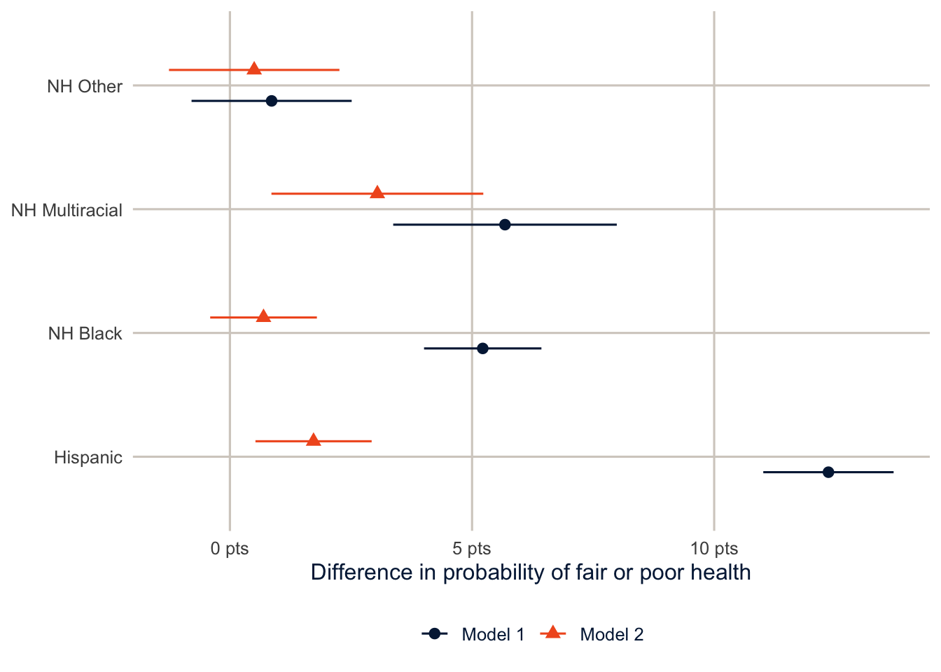
Now the result reads in percentage points, which is what most readers think in anyway. Before adjusting for SES, Hispanic adults are 12.4 percentage points more likely than non-Hispanic White adults to report fair or poor health. After adjustment the gap is 1.7 points. I’d report the AMEs next to (or in place of) the odds ratios in a paper, and I’ll expect them in yours.
AMEs fix the scale problem, but not the interpretation problem. Both AMEs here are averaged over the same people (the complete-case sample, with the same weights), which is what makes them comparable; if the two models were fit to different samples, the comparison would mix in the difference between the samples. And the drop from one to the other describes how the race difference changes when we compare people with the same education and income. It doesn’t show that education and income cause that part of the difference.
TipReading the result: a right and a wrong interpretation
Right: “Comparing adults of the same age and sex, Hispanic adults are 12.4 percentage points more likely than non-Hispanic White adults to report fair or poor health. Among adults who also have the same education and income, the difference is 1.7 points.”
Wrong: “Education and income explain 84% of the Hispanic health disadvantage.” That number is the naive change in the logit coefficient, which mixes in rescaling, and “explain” implies a causal story (that the disadvantage runs through SES) the model can’t establish.
Stratified models
You’ll often see models in the literature stratified by some predictor, fit separately for men and women, say, or for each racial and ethnic group. This is usually because the hypothesis is that the effect of one variable differs across the groups. Does education protect everyone’s health equally, or does it pay off more for some groups than others?
The first thing to do is test the interaction. If the education by race interaction isn’t significant, we have no justification for stratifying, because the data don’t tell us the effect of education varies by race. This is the test of parallel slopes from the analysis of covariance.
m_int <- svyglm(badhealth ~ race_eth * educ + agec + female + income + smoke + insured,
                design = des_cc, family = quasibinomial())
regTermTest(m_int, ~ race_eth:educ, method = "Wald")
#> Wald test for race_eth:educ
#> in svyglm(formula = badhealth ~ race_eth * educ + agec + female +
#> income + smoke + insured, design = des_cc, family = quasibinomial())
#> F = 2.359678 on 12 and 168737 df: p= 0.0049746In a formula, race_eth * educ means “both variables and their interaction”: R adds race_eth, educ, and every product of a race dummy with an education dummy. The interaction terms alone are written race_eth:educ, which is what regTermTest() tests here.
The interaction test gives p = 0.005, so there is evidence that the education gradient isn’t the same in every group. Now we can stratify. I fit the model separately for non-Hispanic White, non-Hispanic Black and Hispanic adults by subsetting the design.
groups <- c("NH White", "NH Black", "Hispanic")

strat <- groups |>
  set_names() |>
  map(\(g) svyglm(badhealth ~ educ + agec + female + income + smoke + insured,
                  design = subset(des_cc, race_eth == g),
                  family = quasibinomial()))

modelsummary(strat, coef_omit = "agec|Intercept",
             coef_rename = \(x) str_remove_all(x, "educ|income|smoke"),
             gof_map = "nobs", fmt = 3,
title = "Logit coefficients for fair or poor health, stratified by race and ethnicity")| NH White | NH Black | Hispanic | |
|---|---|---|---|
| HS graduate | -0.540 | -0.127 | -0.378 |
| (0.080) | (0.146) | (0.092) | |
| Some college | -0.525 | -0.294 | -0.508 |
| (0.079) | (0.147) | (0.105) | |
| College graduate | -0.977 | -0.453 | -0.964 |
| (0.081) | (0.158) | (0.111) | |
| female | 0.001 | 0.185 | 0.039 |
| (0.034) | (0.077) | (0.074) | |
| $25k-$50k | -0.607 | -0.582 | -0.482 |
| (0.053) | (0.101) | (0.084) | |
| $50k-$100k | -1.201 | -1.068 | -0.779 |
| (0.052) | (0.107) | (0.111) | |
| $100k+ | -1.730 | -1.562 | -1.315 |
| (0.060) | (0.136) | (0.137) | |
| Former | 0.401 | 0.418 | 0.252 |
| (0.038) | (0.109) | (0.096) | |
| Current | 0.635 | 0.494 | 0.387 |
| (0.050) | (0.105) | (0.118) | |
| insured | 0.107 | -0.100 | -0.164 |
| (0.081) | (0.175) | (0.089) | |
| Num.Obs. | 120125 | 16903 | 21332 |
To test whether one coefficient is the same in two separate models \(j\) and \(k\), the classic approach (Allison 1999) is a \(z\) test built from the two coefficients and their standard errors, which works because the two groups are independent subsamples:
\[ z = \frac{\beta_{j} - \beta_{k}}{\sqrt{\left[s.e.(\beta_{j})\right]^2 + \left[s.e.(\beta_{k})\right]^2}} \]
z_test <- function(m_j, m_k, term) {
  d <- coef(m_j)[[term]] - coef(m_k)[[term]]
  se <- sqrt(SE(m_j)[[term]]^2 + SE(m_k)[[term]]^2)
  tibble(term = term, difference = d, z = d / se, p = 2 * pnorm(-abs(d / se)))
}

bind_rows(z_test(strat[["Hispanic"]], strat[["NH White"]], "educCollege graduate"),
          z_test(strat[["NH Black"]], strat[["NH White"]], "educCollege graduate"))
#> # A tibble: 2 × 4
#> term difference z p
#> <chr> <dbl> <dbl> <dbl>
#> 1 educCollege graduate 0.0132 0.0964 0.923
#> 2 educCollege graduate 0.524 2.96 0.00306z_test() is a small function, like mymean() in week 1, that turns the formula above into code. pnorm(-abs(z)) is the probability of a standard Normal value below \(-|z|\), and doubling it gives the two-sided p-value. bind_rows() stacks the two one-row results. In the stratified models above, subset(des_cc, race_eth == g) restricts the design to one group at a time inside map().
The college coefficient for Hispanic adults isn’t significantly different from the one for non-Hispanic White adults (p = 0.92). The one for Black adults is less negative, and the difference is significant (p = 0.0031), which would usually be read as a college degree being associated with a smaller health advantage for Black adults than for White adults. That’s a finding with a real literature behind it, often discussed as “diminished returns” to education. But here’s the catch, which brings us back to the scaling problem.
Comparing effects across groups
The same scaling problem shows up when you compare a coefficient across groups, for example the education gradient for men versus women in separate models. If the residual variance differs between the groups, the logit coefficients differ even when the underlying effects don’t (Allison 1999). AMEs sidestep this too. Here I fit the model separately for men and women and compare the AME of a college degree (versus a high school diploma) on the probability scale.
educ_ame <- c(Men = 0, Women = 1) |>
  map(\(s) svyglm(badhealth ~ educ + race_eth + agec,
                  design = subset(des, female == s),
                  family = quasibinomial())) |>
  map(\(m) avg_comparisons(m, wts = "(weights)",
                           variables = list(educ = c("HS graduate", "College graduate")))) |>
  map(as_tibble) |>
  list_rbind(names_to = "sex")

educ_ame |> select(sex, estimate, std.error, conf.low, conf.high) |>
knitr::kable(digits = 3)| sex | estimate | std.error | conf.low | conf.high |
|---|---|---|---|---|
| Men | -0.118 | 0.006 | -0.130 | -0.107 |
| Women | -0.129 | 0.006 | -0.141 | -0.117 |
Men and women are separate subsamples, so the difference between the two AMEs has a standard error of roughly \(\sqrt{SE_1^2 + SE_2^2}\):
educ_ame |>
  summarise(difference = diff(estimate),
            se = sqrt(sum(std.error^2))) |>
  mutate(z = difference / se,
         p = 2 * pnorm(-abs(z)))
#> # A tibble: 1 × 4
#> difference se z p
#> <dbl> <dbl> <dbl> <dbl>
#> 1 -0.0107 0.00839 -1.27 0.204diff(estimate) subtracts the first value from the second (women minus men), and sqrt(sum(std.error^2)) is the formula above.
Compared with a high school diploma, a college degree goes with a probability of fair or poor health that is 11.8 points lower for men and 12.9 points lower for women. The difference between the two is small and not statistically significant, and because both are on the probability scale, that comparison means what it says.
Part 2: Logistic regression for prediction
This part is an introduction. Week 15 builds on every piece of it with more flexible models, so aim to understand the logic here (fit on some data, judge on other data, and decide what “good” means for your purpose) rather than every function.
Explanation versus prediction
Everything so far has been about the coefficients. In prediction we flip that around. The question is how well a model sorts new cases into the right category, and a model can predict well with coefficients that mean nothing causally, or predict badly with coefficients that are perfectly good estimates. Demographers do more prediction than we sometimes admit: imputing missing values, building propensity scores (week 14) and flagging likely nonrespondents all depend on it.
The key rule is that you judge a predictive model on data it wasn’t fit to. A model always looks better on its own training data, and how much better depends on how flexible it is.
The data
For this part I’ll use the DHS model dataset. It looks like a real Demographic and Health Survey but describes no real country, so it’s free to use. The outcome is whether a woman currently uses a modern contraceptive method, among women who are sexually active and not pregnant.
dhs <- get_dhs_model() |>
  filter(v213 == 0, v536 %in% 1:3) |>
  mutate(modern = factor(if_else(v313 == 3, "yes", "no"), levels = c("yes", "no")),
         age = v012,
         children = v218,
         educ = factor(v106, 0:3, c("None", "Primary", "Secondary", "Higher")),
         wealth = factor(v190, 1:5, c("Poorest", "Poorer", "Middle", "Richer", "Richest")),
         rural = factor(v025, 1:2, c("Urban", "Rural")),
         region = factor(v024)) |>
  select(modern, age, children, educ, wealth, rural, region)

count(dhs, modern) |> mutate(share = n / sum(n))
#> # A tibble: 2 × 3
#> modern n share
#> <fct> <int> <dbl>
#> 1 yes 1761 0.259
#> 2 no 5044 0.741filter(v213 == 0, v536 %in% 1:3) keeps women who aren’t pregnant and were sexually active recently. The factor(v106, 0:3, c(...)) calls are the factor(x, levels, labels) pattern from week 2 with the argument names left off; R matches them by position. select() keeps only the variables the model will use.
I put “yes” first because yardstick treats the first factor level as the event of interest. I’m also ignoring the survey design in this part. That’s common in prediction work, because the goal is to sort individuals, not to estimate a population quantity. But if you want performance measures that describe the population (say, sensitivity among all women in the country), you’d use the weights, and tidymodels supports case weights for that.
Training and test data
initial_split() holds out 20% of the data as a test set that we won’t touch until the very end. Stratifying the split on the outcome keeps the share of modern method users the same in both pieces.
set.seed(7283)
dhs_split <- initial_split(dhs, prop = 0.8, strata = modern)
dhs_train <- training(dhs_split)
dhs_test <- testing(dhs_split)
initial_split() decides which rows go where, at random (hence set.seed()), and training() and testing() pull out the two pieces. Here is the whole plan for the data in one picture, so you can see where each piece is used:
flowchart LR
  A["All data"] --> B["Training data<br/>(80%)"]
  A --> C["Test data (20%)<br/>set aside, untouched"]
  B --> D["10 folds"]
  D --> E["Fit on 9 folds,<br/>check on the 10th,<br/>10 times"]
  E --> F["Cross-validated<br/>performance:<br/>choose model and threshold"]
  F --> G["Refit on all<br/>training data"]
  G --> H["Evaluate once<br/>on the test data"]
  C --> H
  classDef data fill:#C8DCFF,stroke:#032044,color:#032044
  classDef step fill:#FFFFFF,stroke:#032044,color:#032044
  classDef final fill:#F15A22,stroke:#032044,color:#032044
  class A,B,C,D data
  class E,F,G step
  class H final
flowchart LR A["All data"] --> B["Training data<br/>(80%)"] A --> C["Test data (20%)<br/>set aside, untouched"] B --> D["10 folds"] D --> E["Fit on 9 folds,<br/>check on the 10th,<br/>10 times"] E --> F["Cross-validated<br/>performance:<br/>choose model and threshold"] F --> G["Refit on all<br/>training data"] G --> H["Evaluate once<br/>on the test data"] C --> H classDef data fill:#C8DCFF,stroke:#032044,color:#032044 classDef step fill:#FFFFFF,stroke:#032044,color:#032044 classDef final fill:#F15A22,stroke:#032044,color:#032044 class A,B,C,D data class E,F,G step class H final
A recipe and a workflow
The model itself is the familiar logit:
\[ \log\left(\frac{\Pr(\text{modern method})}{1 - \Pr(\text{modern method})}\right) = \mathbf{x}'\boldsymbol\beta \quad\Longleftrightarrow\quad \Pr(\text{modern method}) = \frac{1}{1 + \exp(-\mathbf{x}'\boldsymbol\beta)} \]
What’s new is how we use it. Instead of reading the coefficients, we take each woman’s predicted probability and turn it into a predicted class.
A recipe describes the preprocessing (dummy variables, a quadratic for age), a model specification says what kind of model to fit, and a workflow bundles the two so the same steps get applied to every piece of data.
dhs_recipe <- recipe(modern ~ ., data = dhs_train) |>
  step_dummy(all_nominal_predictors()) |>
  step_poly(age, degree = 2)

logit_wf <- workflow(dhs_recipe, logistic_reg())
NoteCode explanation: recipes and workflows
recipe(modern ~ ., data = dhs_train)saysmodernis the outcome and every other column (the.) is a predictor.step_dummy(all_nominal_predictors())turns every factor predictor into dummy variables, the same thingglm()does behind the scenes.step_poly(age, degree = 2)replaces age with age and age squared (in a numerically stable form), so the probability can rise and then fall with age.logistic_reg()is the model specification: an ordinary logit.workflow(recipe, model)bundles the two, so every time the model is fit (on each fold, and at the end), the same preparation is done first, using only the data it’s being fit to.
Cross-validation
To get an honest estimate of performance without touching the test set, we use 10-fold cross-validation on the training data. The data are split into 10 pieces, and the model is fit 10 times, each time on 9 pieces and evaluated on the one left out.
dhs_folds <- vfold_cv(dhs_train, v = 10, strata = modern)

dhs_metrics <- metric_set(roc_auc, brier_class, accuracy, sensitivity, specificity)

logit_cv <- fit_resamples(logit_wf, resamples = dhs_folds, metrics = dhs_metrics,
                          control = control_resamples(save_pred = TRUE))

collect_metrics(logit_cv)
#> # A tibble: 5 × 6
#> .metric .estimator mean n std_err .config
#> <chr> <chr> <dbl> <int> <dbl> <chr>
#> 1 accuracy binary 0.746 10 0.00388 pre0_mod0_post0
#> 2 brier_class binary 0.172 10 0.00169 pre0_mod0_post0
#> 3 roc_auc binary 0.711 10 0.00686 pre0_mod0_post0
#> 4 sensitivity binary 0.231 10 0.00686 pre0_mod0_post0
#> 5 specificity binary 0.925 10 0.00533 pre0_mod0_post0
NoteCode explanation: cross-validation
vfold_cv(dhs_train, v = 10, strata = modern) splits the training data into 10 folds, each with about the same share of users. metric_set() lists the performance measures to compute. fit_resamples() fits the workflow 10 times, once per fold, and computes the metrics on each held-out fold; control_resamples(save_pred = TRUE) keeps the held-out predictions so we can look at them later. collect_metrics() averages each metric over the 10 folds (mean) and gives its standard error.
Before the list, it helps to know that these metrics answer three different questions, and a model can do well on one and badly on another:
- Discrimination: does the model give higher probabilities to the women who use a modern method than to those who don’t? (AUC)
- Calibration: when the model says 30%, do about 30% of those women use one? (the Brier score, partly, and the calibration plot below)
- Classification at a threshold: once we turn probabilities into yes/no predictions with a cutoff, how many of each kind of mistake do we make? (accuracy, sensitivity, specificity)
In detail:
- Accuracy is the share classified correctly at a threshold of 0.5.
- Sensitivity is the share of modern method users the model catches.
- Specificity is the share of non-users it correctly leaves alone.
- The area under the ROC curve (AUC) is the probability that a randomly chosen user gets a higher predicted probability than a randomly chosen non-user. It doesn’t depend on any threshold.
- The Brier score is the mean squared difference between the predicted probability and the 0/1 outcome, so lower is better.
Here is the humbling part. Accuracy is 74.6%, which sounds fine until you notice that only 25.9% of women use a modern method. A “model” that predicts “no” for everyone would be right 74.1% of the time. Our model barely beats that, and its sensitivity is 23.1%, so it misses most users. The AUC of 0.71 says the model does carry real information. The 0.5 threshold is just a bad way to use it when the outcome is this uncommon.
Decision rules and the confusion matrix
It helps to see where those numbers come from. The model gives each woman a probability. To turn probabilities into classes, we need a decision rule: a threshold, so that a woman is classified as a modern method user if \(\Pr(y = \text{modern} \mid \mathbf{x}) > c\), and as a non-user otherwise. The default is \(c = 0.5\). Cross-tabulating the observed classes against the predicted ones gives the confusion matrix.
cv_class <- collect_predictions(logit_cv) |>
  mutate(pred_05 = factor(if_else(.pred_yes > 0.5, "yes", "no"), levels = c("yes", "no")),
         pred_mean = factor(if_else(.pred_yes > base_rate, "yes", "no"),
                            levels = c("yes", "no")))

conf_mat(cv_class, truth = modern, estimate = pred_05)
#> Truth
#> Prediction yes no
#> yes 325 301
#> no 1083 3734collect_predictions() gathers the held-out predictions from all 10 folds into one data frame, with each woman’s predicted probability of “yes” in .pred_yes. The mutate() turns those into predicted classes with two different thresholds, and conf_mat() cross-tabulates the true classes against the predicted ones.
The columns are the truth and the rows are the predictions. The diagonal holds the women the model gets right, the true positives (users predicted to be users) and true negatives (non-users predicted to be non-users). The off-diagonal cells are the mistakes: false positives, non-users the model calls users, and false negatives, users it misses. Accuracy is the diagonal divided by the total. Sensitivity is the true positives divided by all actual users (the first column), and specificity is the true negatives divided by all actual non-users (the second column). With the 0.5 rule, most of the users end up in the false negative cell.
A simple alternative is to use the mean of the outcome as the threshold, calling a woman a likely user if her predicted probability is higher than the share of users in the training data.
conf_mat(cv_class, truth = modern, estimate = pred_mean)#> Truth
#> Prediction yes no
#> yes 886 1220
#> no 522 2815bind_rows(
"Threshold 0.5" = metric_set(accuracy, sensitivity, specificity)(cv_class, truth = modern,
estimate = pred_05),
"Threshold = mean" = metric_set(accuracy, sensitivity, specificity)(cv_class, truth = modern,
estimate = pred_mean),
.id = "rule") |>
select(rule, .metric, .estimate) |>
pivot_wider(names_from = .metric, values_from = .estimate)#> # A tibble: 2 × 4
#> rule accuracy sensitivity specificity
#> <chr> <dbl> <dbl> <dbl>
#> 1 Threshold 0.5 0.746 0.231 0.925
#> 2 Threshold = mean 0.680 0.629 0.698Lowering the threshold trades specificity for sensitivity. The model now catches far more of the users, at the cost of flagging more non-users, and overall accuracy falls. Which rule is better depends entirely on what the predictions are for.
Choosing a threshold
The threshold is a decision, not a statistical result, and it should reflect what the two kinds of error cost. A program trying to reach every woman with an unmet need for family planning might accept a lot of false positives to avoid missing anyone. probably::threshold_perf() shows the tradeoff using the cross-validated predictions.
cv_preds <- collect_predictions(logit_cv)

thresholds <- threshold_perf(cv_preds, modern, .pred_yes,
                             thresholds = seq(0.05, 0.75, by = 0.01),
                             metrics = metric_set(sensitivity, specificity, j_index))

best_j <- thresholds |>
  filter(.metric == "j_index") |>
  slice_max(.estimate, n = 1, with_ties = FALSE)

thresholds |>
  ggplot(aes(x = .threshold, y = .estimate, colour = .metric, linetype = .metric)) +
  geom_line(linewidth = 1) +
  geom_vline(xintercept = best_j$.threshold, colour = utsa_cols("smoke")) +
  scale_colour_utsa() +
  labs(x = "Threshold", y = "Estimate", colour = NULL, linetype = NULL)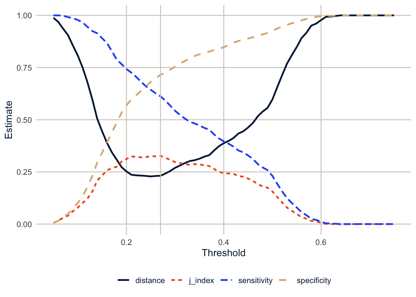
Youden’s J, which weights sensitivity and specificity equally, peaks at a threshold of 0.27. That’s close to the share of users in the data, which is a common and sensible starting point when the outcome is uncommon. But it’s a statistical criterion, not a decision. Youden’s J assumes missing a user and wrongly flagging a non-user are equally bad. If they aren’t (and for most real programs they aren’t), the best threshold for the program is somewhere else, and choosing it means deciding how much each kind of mistake costs.
threshold_perf() computes the chosen metrics at each threshold in thresholds, and slice_max(.estimate, n = 1) keeps the row with the highest J.
Calibration
A model can rank people well and still get the probabilities wrong. Calibration asks whether, among women with a predicted probability around 0.3, about 30% actually use a modern method. If the predicted probabilities are going to be used as probabilities (as risk scores, or in propensity score weights in week 14), calibration matters as much as discrimination.
cv_preds |>
  mutate(bin = ntile(.pred_yes, 10)) |>
  group_by(bin) |>
  summarise(predicted = mean(.pred_yes),
            observed = mean(modern == "yes"),
            n = n()) |>
  ggplot(aes(x = predicted, y = observed)) +
  geom_abline(colour = utsa_cols("smoke"), linewidth = 1) +
  geom_line(colour = utsa_cols("midnight")) +
  geom_point(colour = utsa_cols("orange"), size = 3) +
  coord_equal(xlim = c(0, 0.7), ylim = c(0, 0.7)) +
  labs(x = "Mean predicted probability", y = "Observed share using a modern method")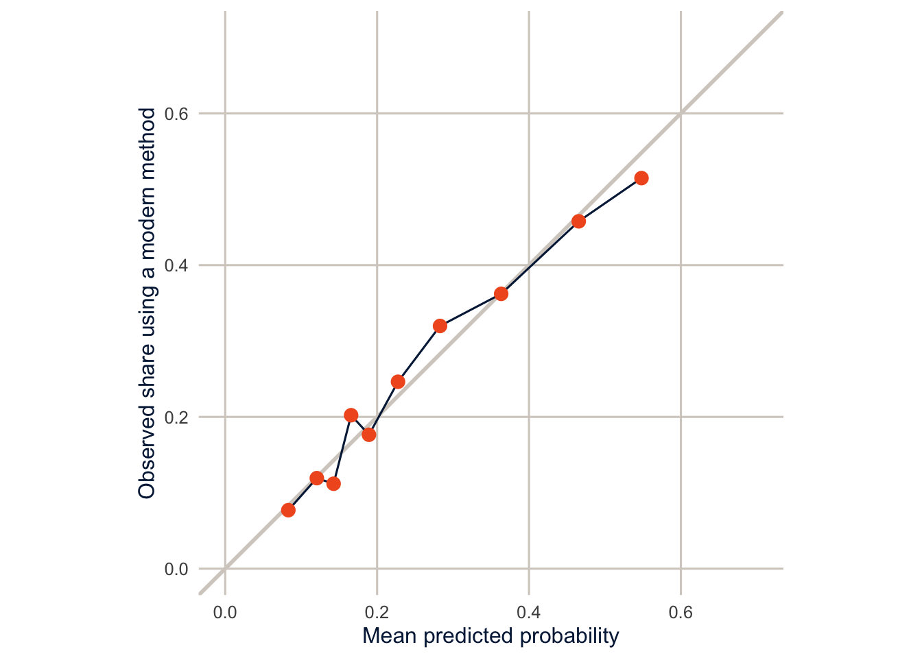
ntile(.pred_yes, 10) sorts the women by predicted probability and splits them into 10 equal-sized groups (deciles). For each decile, the plot compares the average predicted probability with the share who actually use a modern method. geom_abline() draws the diagonal line where the two are equal.
The points sit close to the diagonal, so this model’s probabilities can be taken roughly at face value, on data like these. That’s common for logistic regression fit to a reasonably large sample, but it isn’t guaranteed, so always check calibration on data the model wasn’t fit to. Flexible machine learning models (week 15) often discriminate better and calibrate worse, so check both.
The test set, once
Now, and only now, we fit the final model to all of the training data and evaluate it on the test set. last_fit() does both steps.
final_fit <- last_fit(logit_wf, split = dhs_split, metrics = dhs_metrics)
collect_metrics(final_fit)
#> # A tibble: 5 × 4
#> .metric .estimator .estimate .config
#> <chr> <chr> <dbl> <chr>
#> 1 accuracy binary 0.746 pre0_mod0_post0
#> 2 sensitivity binary 0.224 pre0_mod0_post0
#> 3 specificity binary 0.929 pre0_mod0_post0
#> 4 roc_auc binary 0.733 pre0_mod0_post0
#> 5 brier_class binary 0.167 pre0_mod0_post0last_fit() fits the workflow to all of the training data and evaluates it on the test data, in one step, so you can’t accidentally peek.
The test-set numbers are close to the cross-validated ones, which is what we hope to see. If they had been much worse, that would be a sign of overfitting, or of a test set that differs from the training data in some way. And the rule matters: if you look at the test set, change the model, and look again, it’s no longer a test set.
Warning
A predictive model is only as fair as the data and the decision it feeds. A model that is well calibrated overall can be poorly calibrated for a particular group, and a threshold that looks fine on average can miss most of the people in a group the program most needs to reach. Before a model like this informs anyone’s access to services, check its performance separately by region, wealth and education. Exercise 4 starts on this.
Homework 4
Due: February 18, before class.
Which version to do. If you’re in DEM 7283, do the version with your own survey data. If you’re in DEM 5283, do either version, and say at the top of your homework which one you did. If your survey can’t support this week’s method, do the version with my data and say so.
Purpose. Compare nested models in a way that means what it says, and judge a prediction model by how it will be used.
A satisfactory answer compares models on the probability scale for the same people; describes changes in a comparison as associations, not as what a variable “explains” or “causes”; and, for prediction, says which kind of performance (discrimination, calibration or classification) each number measures.
With your own survey data
Use the full survey design for every estimate unless a step says otherwise, and report each estimate with a standard error or confidence interval.
Part 1: Nested models and interactions
- Use your binary outcome from Homework 3, and choose one key predictor (for example, race and ethnicity, sex, or nativity) whose association with the outcome you want to understand.
- Construct relevant control variables for your outcome, based on the literature in your area of interest, and group them into two sets: basic demographic controls, and variables that might account for part of the key predictor’s association (for example, education and income).
- Fit two nested models: one with the key predictor and basic controls, and one that adds the second set.
- Report the average marginal effects of the key predictor from both models, for the same complete-case sample.
- How does the association change when the second set is added?
- Why can’t you compare the logit coefficients from the two models directly? Use the KHB method to make the comparison on a common scale.
- Examine an interaction between your key predictor and one other predictor.
- Test the interaction terms jointly with
regTermTest(). - Present predicted probabilities that show what the interaction means.
- Test the interaction terms jointly with
- Stratify your model by one predictor.
- What evidence do you use to justify the stratification?
- Is there evidence for homogeneity of regression effects across the strata? How do you know?
- Explain and discuss the implications, interpreting the models both within and between the strata.
Part 2: Prediction
- Treat your outcome as something to predict, rather than explain. Split your data into training and test sets, and fit a logistic regression on the training data with
tidymodels. - Use 10-fold cross-validation on the training data to estimate how well the model predicts.
- On the test data, report:
- the area under the ROC curve (discrimination);
- a calibration plot (calibration); and
- the sensitivity and specificity at a threshold you choose, and why you chose it (classification).
- In two or three sentences, explain why a good model for explanation (Part 1) isn’t necessarily a good model for prediction, and the reverse.
With my data
What is provided. The BRFSS data with recode_mmsa(), the complete-case design des_cc, and the code for Models 1 and 2 from this chapter; the DHS prediction data, split, folds and workflow from Part 2.
1. Repeat the nested comparison for obesity (obese) as the outcome, using Models 1 and 2 (age and sex, then add education and income). Report the Hispanic-White and Black-White average marginal effects from both models, in percentage points, for the same complete-case sample. Describe how each estimated difference changes when education and income are added. Then, in two or three sentences, explain why a coefficient that shrinks when variables are added doesn’t by itself show that those variables mediate the difference. (Optional: also report the naive and KHB changes in the logit coefficients, and say whether rescaling is bigger or smaller than it was for self-rated health.)
# YOUR CODE HERE2. (Optional.) Get a standard error for the KHB change in the Hispanic coefficient. Restrict the data to the Texas metro areas, convert the design to 100 bootstrap replicates with as.svrepdesign(), and repeat the KHB calculation within each replicate using withReplicates() or a loop over the replicate weights.
# YOUR CODE HEREA hint for exercise 2
After rep_des <- as.svrepdesign(...), weights(rep_des, "analysis") gives you a matrix of replicate weights with one column per replicate. Fit the residualizing regressions and both logit models with each column as the weight (glm() with weights = gives the same point estimates as svyglm()), save the change for each replicate, and take the standard deviation, scaled as svrVar() would.
3. Add wealth by residence (wealth * rural) and the number of children ever born (v201) to the DHS prediction model. Does the cross-validated AUC improve? What about the Brier score?
# YOUR CODE HERE4. Using the cross-validated predictions from the final model, compute sensitivity and specificity at the Youden threshold separately for urban and rural women. Write two or three sentences about what the difference would mean for a program that used this model to target outreach.
# YOUR CODE HERE5. Suppose the model in exercise 3 predicted modern method use very well (an AUC of 0.90). Would that tell you why wealthier women are more likely to use modern methods? In two or three sentences, explain the difference between a model that predicts well and a model that explains a difference between groups.
Additional resources
- Breen et al. (2018), in the Annual Review of Sociology, reviews the scaling problem, KHB, and the case for marginal effects, and it’s the paper to cite when a reviewer asks why you didn’t just compare the coefficients.
- Mood (2010) is the shorter and more pointed version of the same argument, and still the most-cited one.
- Tidy Modeling with R (Kuhn and Silge 2022), free online, covers resampling, cross validation and performance metrics with
tidymodels. Week 15 builds on it.