Week 15: Tree-Based Machine Learning with tidymodels

Introduction

Almost everything this semester has been about explanation: estimating how an outcome is related to particular predictors, with standard errors, so we can say something about the population. Week 4 introduced a different goal, prediction: getting the outcome right for people the model hasn’t seen. Machine learning methods are built for prediction, and they’ve become common in social science (Molina and Garip 2019), for imputing missing data, targeting services, and screening for risk, among other things.

This week covers tree-based methods (classification trees, random forests and boosted trees) using the tidymodels framework (Kuhn and Silge 2022), and three things that matter as much as the algorithm: honest evaluation with cross-validation, calibration (do the predicted probabilities mean what they say?), and fairness (does the model work equally well for everyone?). The last one is where a demographer’s training is most useful, and where prediction for policy can go wrong.

NoteThis week at a glance

The question. If a health department wanted to flag adults in fair or poor health for outreach, using a short intake questionnaire, how well could a model do it, and would it work equally well for everyone?

By the end of this week you should be able to

1. define a prediction task (who is predicted, when, and for what decision), and say which predictors would be available at that time;
2. explain how trees, random forests and boosted trees work, and tune and compare them against a logit baseline with cross-validation and a test set;
3. evaluate a model’s discrimination, calibration and decision consequences separately, overall and for subgroups, with appropriate caution.

Before you begin. You need everything in Part 2 of week 4: training and test data, cross-validation, the confusion matrix and calibration. This week goes deeper into each one.

Required and optional. Everything is required, but the code that draws the trees, forests and boosting figures is there to show the ideas; you won’t need to write code like it.

Setup

library(tidyverse)
library(here)
library(tidymodels)
library(rpart.plot)    # draws classification trees (also loads rpart)
library(sparkscolors)  # pak::pak("coreysparks/sparkscolors"), UTSA colors

source(here("R", "get_mmsa.R"))
source(here("R", "recode_mmsa.R"))

tidymodels_prefer()

NoteCode explanation: tidymodels and tidymodels_prefer()

tidymodels is a collection of packages that work together, the way the tidyverse is: rsample splits data, recipes prepares predictors, parsnip specifies models, workflows bundles a recipe and a model, tune tunes, and yardstick measures performance. Several of its function names clash with functions in other packages (dplyr and MASS both have a select(), for example). tidymodels_prefer() tells R to use the tidymodels version whenever there’s a conflict, which saves a lot of confusing error messages.

Prediction is a different goal

When we explain, we care about the coefficients: their size, their sign, and their standard errors. When we predict, we care about the predictions, and the coefficients are just a means to an end. That changes three things.

1. We judge a model on new data. A model can fit the data it was estimated on very well and predict new data badly, because it has learned the noise. That’s overfitting, and the only protection is to test the model on data it hasn’t seen.
2. Flexibility is a tool, not a risk to avoid. A model with thousands of interactions and nonlinearities would be uninterpretable as an explanation, but if it predicts better on new data, it’s a better predictive model.
3. Prediction is not causation. A variable that predicts an outcome may do so because it causes it, because the outcome causes it, or because both share a cause. For prediction, it doesn’t matter. For deciding what to do about the outcome, it matters enormously (that was week 14).

Trees

Random forests and boosted trees are both built out of a simpler model, the classification tree, so we start there. The plan for this part of the lesson is: grow one tree and see how it works, see why one tree on its own isn’t very good, and then look at the two ways of combining many trees to fix that.

Classification trees

A classification tree predicts an outcome by asking a series of yes-or-no questions about a person, like the game twenty questions. “Did you have 9 or more days of poor physical health last month? If so, was it 15 or more? Are you unable to work?” Each answer sends the person down one branch of the tree, and they end up in a final group, called a leaf. The prediction for everyone in a leaf is the share of people in that leaf, in the data the tree was grown on, who have the outcome. There are no coefficients and no equation, just the questions.

Compare that with the logit models you know. A logit model assumes each predictor has the same effect on the log-odds for everybody (unless you add interactions yourself) and that a continuous predictor has a straight-line effect (unless you add polynomials or splines yourself, as in week 11). A tree assumes neither. Because each question is asked only within the group created by the earlier questions, a tree finds interactions on its own, and because it can ask about the same variable several times with different cut points, it finds nonlinear relationships on its own too.

Data

A prediction model should start from how it will be used, because that decides what “good” means. Here’s the task for this chapter:

Who is predicted	Adults living in the BRFSS SMART metro areas
When the prediction is made	At a short intake interview, when the person answers a few questions about themselves and their recent health
What decision it supports	Whether a health department flags the person for a follow-up outreach call
Which mistakes matter	Missing someone in poor health (a false negative) means no call; flagging someone in good health (a false positive) uses up a call

I’ll predict fair or poor self-rated health in the 2024 BRFSS, from demographics, socioeconomic status, health behaviors, and the numbers of poor physical and mental health days. To keep the run time reasonable, I take a random sample of 20,000 respondents with complete data.

One rule follows straight from the task: a predictor has to be available when the prediction is made. At an intake interview, someone can tell you how many bad health days they had last month, so phys_days and ment_days are fair game for this task. They’re measured at the same time as the outcome and are almost measures of it, though, so the same model would be useless for forecasting who will be in poor health next year, before any of that is known. Exercise 2 shows how much the model leans on them.

Two other limits to keep in mind. The model is trained and judged on respondents with complete data, unweighted, so its performance numbers describe that sample, not necessarily the adult population of these metros (week 9’s and week 2’s problems, again). And a random split of respondents tells you how the model does on new people like these, from the same metros in the same year. It doesn’t tell you how it would do in a different metro, a later year, or a different population, which is often what you’d actually want to know.

set.seed(7283)
brfss <- get_mmsa() |>
  recode_mmsa() |>
  mutate(badhealth = factor(badhealth, levels = c(1, 0), labels = c("Fair/poor", "Good+")),
         age = age80,
         employed = factor(case_when(employ1 %in% 1:2 ~ "Employed",
                                     employ1 %in% 3:4 ~ "Unemployed",
                                     employ1 %in% 5:6 ~ "Homemaker or student",
                                     employ1 == 7 ~ "Retired",
                                     employ1 == 8 ~ "Unable to work")),
         exercise = case_when(exerany2 == 1 ~ 1, exerany2 == 2 ~ 0)) |>
  select(badhealth, age, female, race_eth, educ, income, insured, smoke, bmi,
         ment_days, phys_days, employed, exercise) |>
  drop_na() |>
  slice_sample(n = 20000)

count(brfss, badhealth) |> mutate(share = n / sum(n))

#> # A tibble: 2 × 3
#>   badhealth     n share
#>   <fct>     <int> <dbl>
#> 1 Fair/poor  3417 0.171
#> 2 Good+     16583 0.829

NoteCode explanation: the outcome as a factor

tidymodels classification models need the outcome to be a factor, and by default they treat the first level as the event of interest. That’s why I put "Fair/poor" first. Get this backward, and the ROC AUC will come out as 1 minus the right answer.

Splitting the data

The first step in any predictive analysis is to set aside a test set that you don’t touch until the very end. Everything else (choosing a model, tuning it) happens on the training set, using cross-validation: split the training data into \(v\) folds, fit the model on \(v - 1\) of them, evaluate it on the one left out, and repeat until every fold has been left out once.

split <- initial_split(brfss, prop = 0.75, strata = badhealth)
train <- training(split)
test <- testing(split)
folds <- vfold_cv(train, v = 5, strata = badhealth)

Here’s how the pieces are used, the same plan as in week 4, now with a tuning step:

flowchart LR
  A["All data"] --> B["Training data<br/>(75%)"]
  A --> C["Test data (25%)<br/>set aside, untouched"]
  B --> D["5 folds"]
  D --> E["For each candidate model<br/>and tuning value: fit on 4 folds,<br/>check on the 5th, 5 times"]
  E --> F["Choose the model<br/>and tuning values"]
  F --> G["Refit on all<br/>training data"]
  G --> H["Evaluate once<br/>on the test data"]
  C --> H
  classDef data fill:#C8DCFF,stroke:#032044,color:#032044
  classDef step fill:#FFFFFF,stroke:#032044,color:#032044
  classDef final fill:#F15A22,stroke:#032044,color:#032044
  class A,B,C,D data
  class E,F,G step
  class H final

flowchart LR
  A["All data"] --> B["Training data<br/>(75%)"]
  A --> C["Test data (25%)<br/>set aside, untouched"]
  B --> D["5 folds"]
  D --> E["For each candidate model<br/>and tuning value: fit on 4 folds,<br/>check on the 5th, 5 times"]
  E --> F["Choose the model<br/>and tuning values"]
  F --> G["Refit on all<br/>training data"]
  G --> H["Evaluate once<br/>on the test data"]
  C --> H
  classDef data fill:#C8DCFF,stroke:#032044,color:#032044
  classDef step fill:#FFFFFF,stroke:#032044,color:#032044
  classDef final fill:#F15A22,stroke:#032044,color:#032044
  class A,B,C,D data
  class E,F,G step
  class H final

Training, tuning and testing. Every choice (which model, which tuning values, which threshold) is made with cross-validation on the training data. The test set is used once, at the end.

strata = badhealth makes sure each piece has the same share of people in fair or poor health, which matters when the outcome is uncommon.

Growing one tree

Here is how a tree is grown, in words.

1. Start with everyone in a single group.
2. Consider every possible yes-or-no question: for every predictor, every place you could cut it in two. For age, that’s “under 19 or 19 and over?”, “under 20 or 20 and over?”, and so on. For a categorical variable like income, it’s every way of dividing the categories into two sets.
3. Pick the question that does the best job of separating people in fair or poor health from people in good health, and split the group in two.
4. Repeat steps 2 and 3 inside each of the two new groups, and inside the groups they make, and so on, until a stopping rule says to stop. Here, the rule is that no one can be more than three questions from the top (a depth of 3).

spec_tree <- decision_tree(tree_depth = 3, cost_complexity = -1) |>
  set_mode("classification")

tree_fit <- fit(spec_tree, badhealth ~ ., data = train)

NoteCode explanation: fitting one tree

1. decision_tree() is the parsnip specification for a single tree. Its default engine is the rpart package (“recursive partitioning”, which is another name for growing a tree). set_mode("classification") says the outcome is categorical.
2. tree_depth = 3 is the stopping rule from step 4. cost_complexity is a second stopping rule, which stops a split unless it improves the fit by a given amount. I’ve switched it off (-1) so you can see the full depth-3 tree; we’ll come back to stopping rules below.
3. fit(spec, formula, data) fits a model specification directly, without a recipe or workflow. That’s fine here because rpart handles factors on its own, and leaving them as factors makes the tree easier to read than dummy variables would.

node_label <- function(x, labs, digits, varlen) {
  paste0(round(100 * x$frame$yval2[, 4]), "% fair/poor\nn = ", trimws(fmt(x$frame$n)))
}
split_label <- function(x, labs, digits, varlen, faclen) {
  str_replace(labs, "Under \\$25k,\\$25k-\\$50k", "under $50k")
}

rpart.plot(extract_fit_engine(tree_fit), type = 2, roundint = FALSE,
           node.fun = node_label, split.fun = split_label,
           box.palette = c(utsa_cols("orange")[[1]], utsa_cols("mission_clay")[[1]],
                           utsa_cols("limestone")[[1]]),
           col = utsa_cols("midnight")[[1]], split.col = utsa_cols("midnight")[[1]],
           branch.col = utsa_cols("smoke")[[1]], shadow.col = 0, varlen = 0, faclen = 0)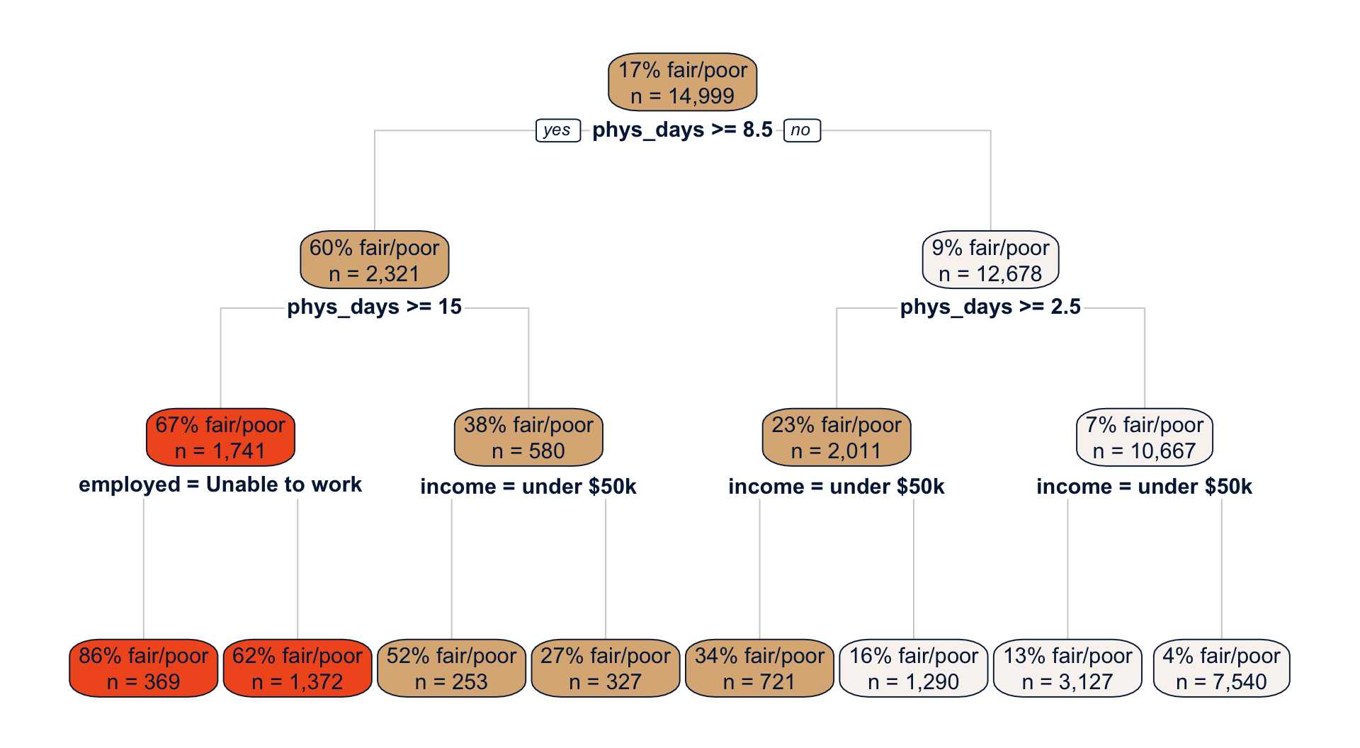

Figure 15.1: A classification tree of depth 3, grown on the training data. Each box gives the share in fair or poor health and the number of people in that group. People who answer “yes” to a question go left.

NoteCode explanation: drawing a tree with rpart.plot()

1. extract_fit_engine() pulls the rpart object out of the parsnip fit, and rpart.plot() draws it. type = 2 puts each question under its box, and roundint = FALSE shows the cut points exactly as rpart stored them.
2. By default the boxes show the predicted class and the share in the second outcome category, which is hard to read. node.fun lets you write the box labels yourself. rpart.plot() hands the function the fitted tree as x; x$frame has one row per box, its column n is the number of people in the box, and column 4 of yval2 is the share in the first outcome category, “Fair/poor”.
3. split.fun does the same for the questions. Mine only shortens the long income label, using str_replace() (the \\$ is needed because $ has a special meaning in a search pattern).
4. box.palette shades the boxes from Orange (mostly fair or poor) to Limestone (mostly good health), and the other col arguments set the text and line colors.

Read the tree from the top. In the training data, 17% of people report fair or poor health. The first question is about poor physical health days, and it divides people into a group with 9 or more days (cut at 8.5), 60% of whom are in fair or poor health, and a much larger group with fewer days, only 9% of whom are. Every later question is asked within one of those groups, and that’s where the tree finds interactions. Among people with many poor health days, being unable to work is the next most useful question. Among people with few, income is. The tree also asks about physical health days twice on each side, at different cut points, which gives it a staircase-shaped, nonlinear relationship between health days and the outcome. No one had to tell it to do either of those things.

To predict for a new person, drop them down the tree and read off their leaf. An 80-year-old with 20 poor health days who is unable to work lands in the leftmost leaf, so the tree predicts an 86% chance that they’re in fair or poor health.

How the tree picks a question

“Best separates” in step 3 needs a number. The most common one is the Gini impurity, which measures how mixed a group is. If a share \(p\) of a group is in fair or poor health, its impurity is \(2p(1 - p)\). That’s 0 when everyone in the group is the same (\(p = 0\) or \(p = 1\)), and at its largest, 0.5, when the group is split half and half. The tree computes the impurity of the two groups a question would create, averages them (weighting by group size), and picks the question that lowers the impurity the most. Here’s the calculation for the first question.

gini <- function(p) 2 * p * (1 - p)
cut1 <- extract_fit_engine(tree_fit)$splits[1, "index"]

impurity <- train |>
  mutate(group = if_else(phys_days >= cut1, paste(cut1, "or more days"),
                         paste("Fewer than", cut1, "days"))) |>
  summarise(n = n(), share = mean(badhealth == "Fair/poor"), .by = group) |>
  mutate(impurity = gini(share))
impurity

#> # A tibble: 2 × 4
#>   group                   n  share impurity
#>   <chr>               <int>  <dbl>    <dbl>
#> 1 8.5 or more days     2321 0.600     0.480
#> 2 Fewer than 8.5 days 12678 0.0923    0.168

c(before = gini(mean(train$badhealth == "Fair/poor")),
  after = weighted.mean(impurity$impurity, impurity$n))

#>    before     after 
#> 0.2832697 0.2159058

NoteCode explanation: computing the impurity by hand

1. gini() is a one-line function for the formula above.
2. extract_fit_engine(tree_fit)$splits is a table of the splits rpart chose, and the "index" column of its first row is the cut point of the first question (8.5 days).
3. The pipe puts each person in one of the two groups that question creates, then computes each group’s size, share in fair or poor health, and impurity. summarise(..., .by = group) is a shortcut for group_by(group) |> summarise(...).
4. The last line compares the impurity of everyone together with the size-weighted average impurity of the two groups.

Before the split, the impurity is 0.283. After it, the average is 0.216. The tree tried every other cut point of every other predictor, and none lowered the impurity more. Then it did the same thing again inside each of the two groups.

Too many questions: overfitting

Why stop at three questions? Why not keep going until every leaf is pure? Because a tree that keeps asking questions eventually stops learning about fair or poor health and starts memorizing the particular people in the training data. With enough questions, it can put almost every person in a leaf of their own and get every one of them right. That’s overfitting, and you can see it happen. Below, I grow trees of increasing depth on four of the five cross-validation folds and check each one in two places: on the data it was grown on, and on the fifth fold, which it never saw.

fit_set <- analysis(folds$splits[[1]])
check_set <- assessment(folds$splits[[1]])

depth_auc <- function(d) {
  tree <- decision_tree(tree_depth = d, cost_complexity = -1, min_n = 2) |>
    set_mode("classification") |>
    fit(badhealth ~ ., data = fit_set)
  bind_rows(
    "Data the tree was grown on" = augment(tree, fit_set) |> roc_auc(badhealth, `.pred_Fair/poor`),
    "Held-out data" = augment(tree, check_set) |> roc_auc(badhealth, `.pred_Fair/poor`),
    .id = "data") |>
    mutate(depth = d)
}
depth_res <- map(1:20, depth_auc) |> list_rbind()

ggplot(depth_res, aes(x = depth, y = .estimate, colour = data, shape = data)) +
  geom_line(linewidth = 1) +
  geom_point(size = 2.5) +
  scale_colour_utsa(palette = "primary") +
  labs(x = "Tree depth (number of questions)", y = "AUC", colour = NULL, shape = NULL)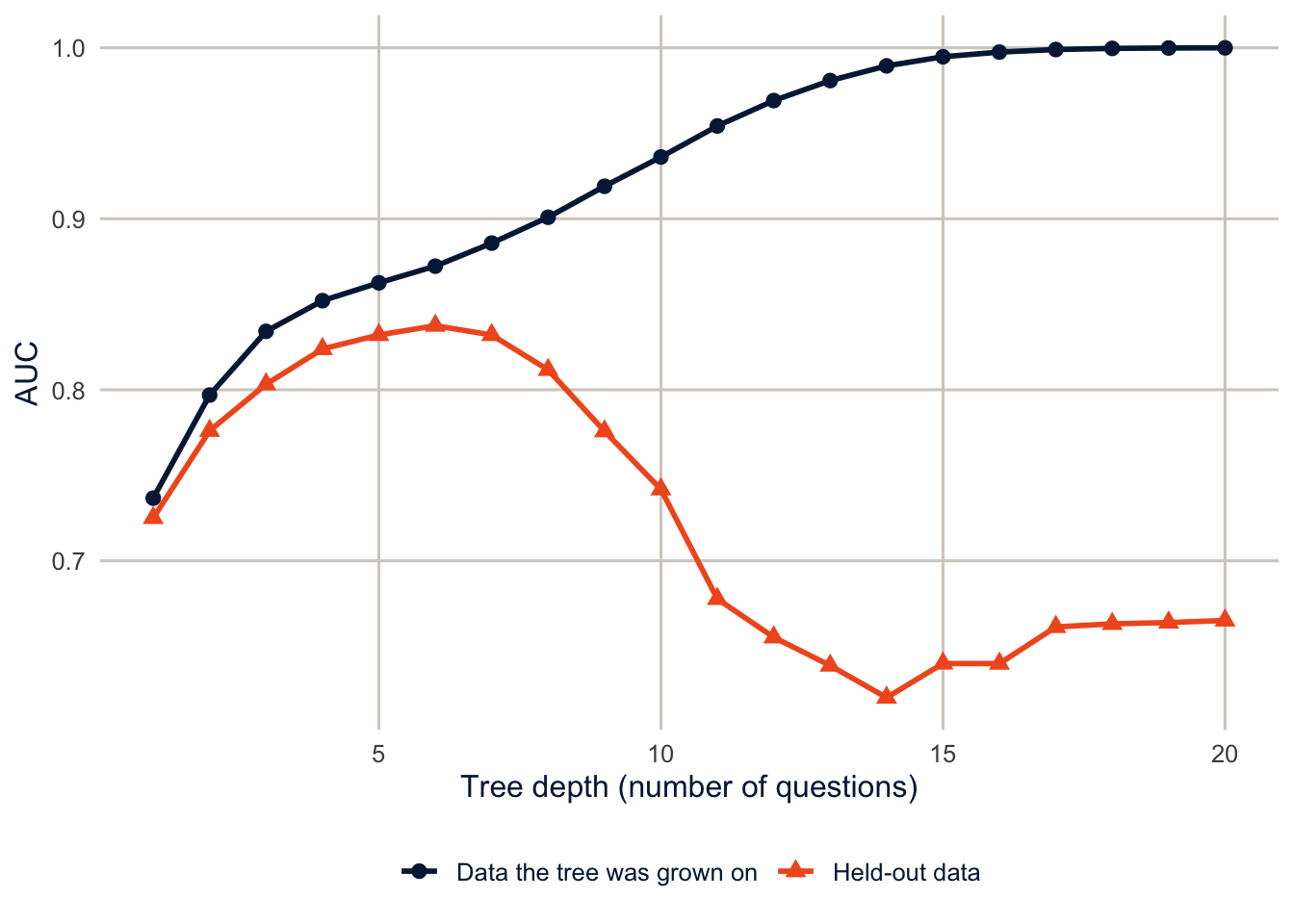

Figure 15.2: AUC of classification trees of increasing depth, on the data they were grown on and on held-out data (one cross-validation fold).

NoteCode explanation: one fold by hand

1. folds$splits[[1]] is the first of the five cross-validation splits. analysis() returns the part used to fit the model (four-fifths of the training data), and assessment() returns the held-out part. fit_resamples() and tune_grid() do this for every fold behind the scenes. Here I do it for one fold so we can see inside.
2. depth_auc() grows a tree of depth d and computes its AUC on both sets. min_n = 2 lets the tree split groups as small as two people, so nothing but the depth stops it.
3. augment(model, data) returns the data with the model’s predictions attached as new columns (.pred_class, .pred_Fair/poor and .pred_Good+), ready to pass to a yardstick metric.
4. map(1:20, depth_auc) |> list_rbind() runs the function for depths 1 to 20 and stacks the results, as in earlier weeks.

On the data it was grown on, the tree keeps getting better as it gets deeper, until a depth-20 tree has an AUC of 1, which is essentially perfect. On new data, it improves up to a depth of about 6 (AUC 0.84) and then gets worse, falling to 0.67. The extra questions are learning noise. This is the most important picture in machine learning, and it’s why we always judge a model on data it hasn’t seen.

A single tree has a second problem, which is related. It’s unstable: draw a slightly different sample, and the first question might change, and then every question below it changes too. A deep tree is very sensitive to the specific people in the training data. Statisticians call this high variance. Random forests and boosted trees are two different ways of combining many trees to fix it.

Random forests: grow many trees and average them

Suppose you ask a crowd to guess how many beans are in a jar. Individual guesses are all over the place, but the average of many guesses is usually closer than almost any one person, as long as people’s mistakes aren’t all the same. A random forest (Breiman 2001) applies that idea to trees.

1. Draw a bootstrap sample of the training data: a sample of the same size, drawn with replacement, so some people appear more than once and others not at all. (This is the same bootstrap you saw as a replication method in week 2.)
2. Grow a deep tree on that sample, with one twist: at each split, the tree may choose only from a small random subset of the predictors (mtry of them), not from all of them.
3. Repeat steps 1 and 2 hundreds of times, so each tree sees a slightly different sample and a different set of predictors.
4. To predict for a person, drop them down every tree and average the trees’ predictions.

Why the twist in step 2? Without it, every tree would ask about physical health days first, and the trees would look much alike and make the same mistakes, and averaging can’t cancel mistakes that everyone makes. Forcing each split to choose from a random few predictors makes the trees different from one another, so their errors partly cancel. (With mtry equal to the number of predictors, there’s no twist, and the method is called bagging, short for bootstrap aggregating.)

Here is a forest of 300 trees grown on the same four folds. The figure shows what each tree predicts for six people in the held-out fold.

set.seed(7283)
rf_demo <- ranger::ranger(badhealth ~ ., data = fit_set, num.trees = 300, probability = TRUE)

set.seed(15)
six <- slice_sample(check_set, n = 6) |>
  mutate(person = paste0("Age ", age, ", ", phys_days, " poor physical health days\n(reported ",
                         if_else(badhealth == "Fair/poor", "fair or poor", "good or better"),
                         " health)"))
each_tree <- predict(rf_demo, data = six, predict.all = TRUE)$predictions[, "Fair/poor", ]

tree_preds <- as_tibble(each_tree, .name_repair = ~ paste0("tree", seq_along(.x))) |>
  mutate(person = six$person) |>
  pivot_longer(-person, names_to = "tree", values_to = "prob") |>
  mutate(person = fct_reorder(person, prob))
forest_preds <- tree_preds |> summarise(prob = mean(prob), .by = person)

ggplot(tree_preds, aes(x = prob, y = person)) +
  geom_point(position = position_jitter(height = 0.2, width = 0, seed = 1),
             alpha = 0.3, colour = utsa_cols("midnight")[[1]], size = 1.5) +
  geom_point(data = forest_preds, shape = 23, size = 5,
             colour = utsa_cols("midnight")[[1]], fill = utsa_cols("orange")[[1]]) +
  scale_x_continuous(labels = scales::label_percent()) +
  labs(x = "Predicted probability of fair or poor health", y = NULL)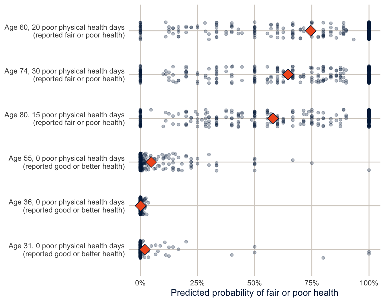

Figure 15.3: Predicted probability of fair or poor health for six people in the held-out fold, from each of the 300 trees in a random forest (dots) and from the forest as a whole (diamonds, the average of the dots).

NoteCode explanation: a forest by hand

1. ranger::ranger() fits a random forest directly with the ranger package, the same engine tidymodels uses below. probability = TRUE asks for predicted probabilities instead of classes. I left mtry at its default, the square root of the number of predictors, rounded down (3 of our 12).
2. slice_sample(n = 6) draws six people at random. set.seed() makes the forest and the draw the same every time the document is rendered.
3. predict(..., predict.all = TRUE) returns every tree’s prediction instead of the average, as an array with one row per person, one column per outcome category and one layer per tree. [, "Fair/poor", ] keeps the “Fair/poor” probabilities, which leaves a table with one row per person and one column per tree.
4. as_tibble() turns that table into a tibble, naming the columns tree1, tree2, and so on, and pivot_longer() makes it one row per person per tree. fct_reorder() sorts the people by their average prediction.
5. position_jitter() moves each dot up or down a little at random so that dots with the same value don’t hide each other. seed = 1 makes the jitter the same each time.

Look at the three people at the top. The individual trees are all over the place: for each of them, some trees say there’s no chance they’re in fair or poor health, others say they certainly are, and many are in between. A single tree is a very noisy guess. The forest’s average, the diamond, is much steadier and more sensible. The more trees in the forest, the more the noise averages out.

forest_auc <- map(c(1, 2, 3, 5, 10, 20, 30, 50, 75, 100, 150, 200, 300), \(k) {
  probs <- predict(rf_demo, data = check_set, num.trees = k)$predictions[, "Fair/poor"]
  tibble(trees = k, auc = roc_auc_vec(check_set$badhealth, probs))
}) |>
  list_rbind()

ggplot(forest_auc, aes(x = trees, y = auc)) +
  geom_hline(yintercept = best_depth$.estimate, colour = utsa_cols("orange")[[1]],
             linetype = "dashed") +
  geom_line(colour = utsa_cols("midnight")[[1]], linewidth = 1) +
  geom_point(colour = utsa_cols("midnight")[[1]], size = 2.5) +
  labs(x = "Number of trees in the forest", y = "Held-out AUC")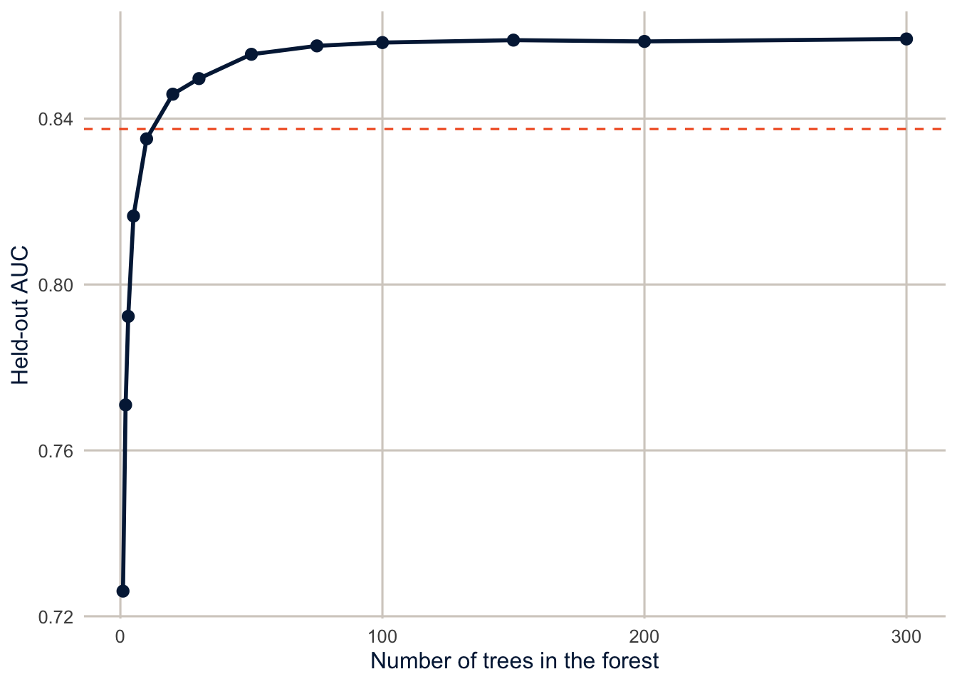

Figure 15.4: Held-out AUC of a random forest using only its first k trees, compared with the best single tree from the previous figure (dashed line).

NoteCode explanation: forests of different sizes

predict(..., num.trees = k) uses only the first k trees of the forest, so one forest gives us forests of every size up to 300. roc_auc_vec() is the version of roc_auc() that takes two vectors (the truth and the probabilities) instead of a data frame and returns a single number.

One tree, grown deep on a bootstrap sample, has a held-out AUC of only 0.73. With 20 trees, the forest already does better than the best single tree we could find by choosing the depth (the dashed line). The curve levels off at about 0.86 after 100 or so trees. Adding more trees to a random forest never makes it worse; it just stops helping, and costs computing time. That’s why the number of trees isn’t something we need to tune. The settings that do matter are mtry, the number of predictors each split may choose from, and min_n, the smallest group the tree is allowed to split, which controls how deep the trees grow.

Boosted trees: many small trees, each fixing the last one’s mistakes

A random forest grows its trees independently and averages them. Boosting (Chen and Guestrin 2016) grows them one after another, and each new tree is aimed at the mistakes of the trees before it. It’s a bit like revising a paper: you don’t rewrite it from scratch each time, you read the reviewers’ comments and fix the parts that are wrong, a little at a time.

1. Start by giving everyone the same prediction: the overall share in fair or poor health.
2. Compute each person’s error: their outcome (1 if they’re in fair or poor health, 0 if not) minus their current prediction.
3. Grow a small tree, only one or a few questions deep, that predicts those errors. In effect, it asks “which people is the model currently getting wrong, and in which direction?”
4. Add a small fraction of that tree’s predictions (the learning rate, for example 0.1) to everyone’s current prediction.
5. Go back to step 2 and repeat, hundreds of times.

The final model is the starting value plus all those small corrections added up. To make this concrete, here is boosting written out by hand, with a single predictor (poor physical health days) and trees with only one question each.

boost_data <- fit_set |>
  transmute(phys_days,
            y = as.numeric(badhealth == "Fair/poor"),
            pred = mean(y))
learn_rate <- 0.1
boost_steps <- list(`0` = boost_data)

for (m in 1:100) {
  boost_data$error <- boost_data$y - boost_data$pred
  small_tree <- rpart(error ~ phys_days, data = boost_data, maxdepth = 1, cp = 0)
  boost_data$pred <- boost_data$pred + learn_rate * predict(small_tree, boost_data)
  if (m %in% c(1, 5, 20, 100)) boost_steps[[as.character(m)]] <- boost_data
}

NoteCode explanation: boosting in a for loop

1. transmute() is mutate() that keeps only the columns it names. boost_data has each person’s health days, their outcome as a 1 or 0 (y), and the starting prediction, the overall share (pred), which is step 1.
2. The for loop repeats its body 100 times, with m counting the rounds (for loops first came up in week 5). Inside the loop:
   • The first line is step 2: each person’s error.
   • The second line is step 3. rpart() grows a regression tree (a tree for a numeric outcome, here the errors) with maxdepth = 1, so it asks a single question, the best place to cut health days in two. A one-question tree is called a stump.
   • The third line is step 4: add a tenth of the stump’s predicted error to everyone’s prediction.
3. The if() line saves a copy of the predictions after rounds 1, 5, 20 and 100, in a list named by the round, so we can plot them.

observed <- fit_set |>
  summarise(share = mean(badhealth == "Fair/poor"), n = n(), .by = phys_days)

boost_steps |>
  list_rbind(names_to = "trees") |>
  mutate(trees = as.numeric(trees),
         panel = if_else(trees == 0, "Start", paste(trees, if_else(trees == 1, "tree", "trees"))),
         panel = fct_reorder(panel, trees)) |>
  distinct(panel, phys_days, pred) |>
  ggplot(aes(x = phys_days)) +
  geom_point(data = observed, aes(y = share, size = n),
             colour = utsa_cols("midnight")[[1]], alpha = 0.5) +
  geom_step(aes(y = pred), colour = utsa_cols("orange")[[1]], linewidth = 1.1) +
  facet_wrap(~ panel, nrow = 1) +
  scale_y_continuous(labels = scales::label_percent()) +
  scale_size_area(max_size = 4, guide = "none") +
  labs(x = "Poor physical health days in the past 30", y = "Share in fair or poor health")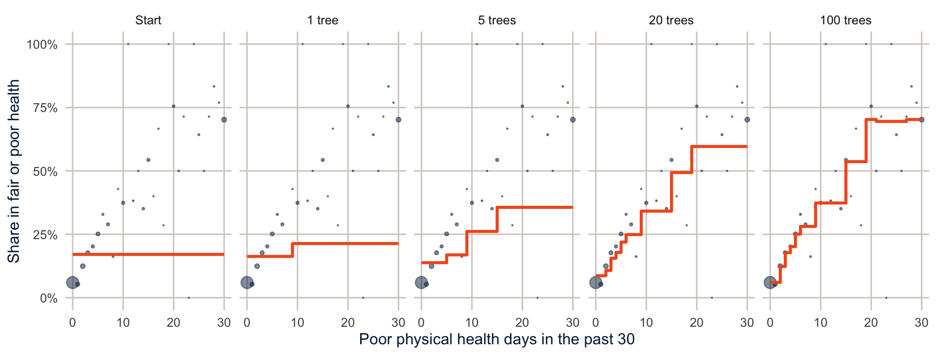

Figure 15.5: Boosting by hand. The line is the model’s predicted probability of fair or poor health at each number of poor physical health days, after 0, 1, 5, 20 and 100 small trees. The dots are the observed shares, sized by the number of people.

NoteCode explanation: plotting the rounds

1. list_rbind(names_to = "trees") stacks the saved copies and adds a column, trees, holding each copy’s name in the list ("0", "1", "5", …). as.numeric() turns those names into numbers so fct_reorder() can put the panels in order.
2. distinct() keeps one row per panel and number of days, since everyone with the same number of days has the same prediction.
3. geom_step() draws the predictions as a staircase, which is the shape a tree’s predictions always have. scale_size_area() sizes the dots by the number of people, so the large group with 0 days stands out.

At the start, everyone gets the overall share, a flat line. The first stump finds the most useful cut in health days and nudges the two sides apart, but only by a tenth of what the stump thinks they should move. Each later stump looks at what’s still wrong and nudges again, adding another step to the staircase. After 100 stumps, the line follows the observed shares closely. Each stump on its own is a terrible model, but together they add up to a good one.

Why such small steps? If each tree corrected the errors completely, the model would chase the noise in the training data and overfit, the same problem as the deep single tree. Small steps make the model learn slowly, so it picks up the patterns that many trees agree on. The cost is that a smaller learning rate needs more trees to get anywhere. That’s the main difference from random forests in practice: with boosting, too many trees can overfit, so the number of trees and the learning rate have to be chosen together, along with tree_depth, how many questions each small tree may ask. The xgboost package we use below does the same thing as this loop, with refinements: it works on the log-odds scale, as a logit model does, it uses all the predictors, and it has extra settings that keep each tree from fitting too closely.

Random forests and boosted trees side by side

	Random forest	Boosted trees
How trees are grown	Independently, each on its own bootstrap sample	One after another, each fit to the errors of the ones before
Size of each tree	Deep (many questions)	Small (a few questions)
How trees are combined	Averaged	Added up, each multiplied by the learning rate
What it fixes	The noise of single deep trees	The bias of single small trees
More trees	Never hurts, eventually stops helping	Can overfit; tune with the learning rate
Main tuning parameters	mtry, min_n	trees, learn_rate, tree_depth

Both are good, general-purpose prediction methods. Random forests work well with little tuning. Boosted trees often predict slightly better when tuned carefully, which is why they win so many prediction competitions, but they’re easier to get wrong.

A recipe and three models

A recipe says how to prepare the predictors. Here, it just turns factors into dummy variables, which the logit model and the boosted trees need. Then I specify three models: a logit model, as a baseline; a random forest; and boosted trees.

rec <- recipe(badhealth ~ ., data = train) |>
  step_dummy(all_nominal_predictors())

spec_logit <- logistic_reg()

spec_rf <- rand_forest(trees = 300, mtry = tune(), min_n = tune()) |>
  set_engine("ranger", importance = "impurity") |>
  set_mode("classification")

spec_xgb <- boost_tree(trees = 300, tree_depth = tune(), learn_rate = tune()) |>
  set_engine("xgboost") |>
  set_mode("classification")

wf_logit <- workflow(rec, spec_logit)
wf_rf <- workflow(rec, spec_rf)
wf_xgb <- workflow(rec, spec_xgb)

NoteCode explanation: model specifications

1. rand_forest() and boost_tree() describe the kind of model, and set_engine() picks the package that fits it (ranger for random forests and xgboost for boosted trees). The same specification could be fit by different engines without changing anything else.
2. tune() marks a tuning parameter, a setting that isn’t estimated from the data by the model itself, so we have to choose it by trying different values and comparing them in cross-validation.
3. workflow(rec, spec) bundles the recipe and the model, so the data preparation is redone inside every fold. That matters: if you prepare the data once using all of it, information from the held-out fold leaks into the training.

The tuning parameters are the settings from the last two sections. For the random forest, mtry is the number of predictors each split may choose from, and min_n is the smallest group a tree may split, which controls how deep the trees grow. I fix the number of trees at 300, since Figure 15.4 showed the forest stops improving well before that. For the boosted trees, learn_rate is the size of each correction and tree_depth is how many questions each small tree may ask. I fix trees at 300 to keep the run time down (exercise 4 asks whether more would help), so the tuning has to find a learning rate that gets far enough in 300 steps.

Tuning and comparing with cross-validation

metrics <- metric_set(roc_auc, brier_class, accuracy)

res_logit <- fit_resamples(wf_logit, folds, metrics = metrics)

res_rf <- tune_grid(wf_rf, folds, grid = 5, metrics = metrics)

xgb_params <- extract_parameter_set_dials(wf_xgb) |>
  update(learn_rate = learn_rate(range = c(-2, -0.5)))  # 0.01 to 0.3, on the log10 scale
res_xgb <- tune_grid(wf_xgb, folds, grid = 5, param_info = xgb_params, metrics = metrics)

NoteCode explanation: tuning

1. fit_resamples() fits a model with nothing to tune once per fold. tune_grid() does the same for each of several candidate values of the tuning parameters (grid = 5 asks for five combinations, spread out over the plausible range).
2. extract_parameter_set_dials() pulls out the tuning parameters and their default ranges, and update() changes one. The default range for learn_rate goes down to 0.0000000001, which, with only 300 trees, gives models that barely learn anything, so I narrowed it.
3. The metrics: ROC AUC is the probability that a randomly chosen person in fair or poor health gets a higher predicted probability than a randomly chosen person in good health, from 0.5 (no better than chance) to 1 (perfect). The Brier score is the mean squared difference between the predicted probability and the outcome, so lower is better, and it rewards good probabilities, not just good rankings. Accuracy is the share classified correctly at a 0.5 threshold, which, as week 4 showed, can be misleading with an uncommon outcome.

bind_rows(
  collect_metrics(res_logit) |> mutate(model = "Logit"),
  show_best(res_rf, metric = "roc_auc", n = 1) |> select(.config) |>
    inner_join(collect_metrics(res_rf), by = ".config") |> mutate(model = "Random forest"),
  show_best(res_xgb, metric = "roc_auc", n = 1) |> select(.config) |>
    inner_join(collect_metrics(res_xgb), by = ".config") |> mutate(model = "Boosted trees")
) |>
  select(model, .metric, mean, std_err) |>
  pivot_wider(names_from = .metric, values_from = c(mean, std_err)) |>
  knitr::kable(digits = 3)

model	mean_accuracy	mean_brier_class	mean_roc_auc	std_err_accuracy	std_err_brier_class	std_err_roc_auc
Logit	0.876	0.093	0.873	0.002	0.001	0.004
Random forest	0.878	0.092	0.874	0.001	0.001	0.004
Boosted trees	0.874	0.094	0.871	0.001	0.001	0.004

The three models predict almost equally well: cross-validated AUCs of 0.873 for the logit, 0.874 for the random forest and 0.871 for boosted trees. That’s a common result with survey data like this. The predictors are a handful of categorical variables and a few counts, and a logit model with main effects captures most of what there is to capture. Tree-based methods shine when there are many predictors, complicated interactions, or strong nonlinearities, and their advantages are often smaller than the hype suggests. Always fit a simple baseline; sometimes it’s the model you should use.

The final model on the test set

Now, and only now, use the test set. I’ll take the boosted trees with their best tuning values, fit them on the whole training set, and evaluate them on the test set, along with the logit for comparison.

final_xgb <- wf_xgb |>
  finalize_workflow(select_best(res_xgb, metric = "roc_auc")) |>
  last_fit(split, metrics = metrics)
final_logit <- last_fit(wf_logit, split, metrics = metrics)

bind_rows(collect_metrics(final_logit) |> mutate(model = "Logit"),
          collect_metrics(final_xgb) |> mutate(model = "Boosted trees")) |>
  select(model, .metric, .estimate) |>
  pivot_wider(names_from = .metric, values_from = .estimate) |>
  knitr::kable(digits = 3)

model	accuracy	roc_auc	brier_class
Logit	0.874	0.866	0.093
Boosted trees	0.874	0.870	0.094

NoteCode explanation: last_fit()

finalize_workflow() plugs the best tuning values into the workflow, and last_fit() fits it to the full training set and evaluates it on the test set in one step. Its name is a reminder: this should be the last thing you fit. If you go back and change the model after seeing the test results, the test set is no longer an honest measure of performance.

From probabilities to classifications: the confusion matrix

Keep three questions apart from here on, because a model can do well on one and badly on another, and whether either is good enough depends on the decision the prediction supports:

1. Discrimination: does the model rank people in fair or poor health above people in good health? The AUC measures this, and only this. A model can rank perfectly while overestimating everyone’s risk.
2. Calibration: are the predicted probabilities right? When the model says 20%, are about 20% of those people in fair or poor health? The Brier score reflects this partly; the calibration plot later in the chapter shows it directly.
3. Decision consequences: once a threshold turns probabilities into “flag” or “don’t flag,” how many of each kind of mistake does the model make, and what do they cost?

The AUC and the Brier score judge the predicted probabilities. But most uses of a model end in a yes-or-no decision: offer the service or don’t, flag the person for follow-up or don’t. To get there, we need a decision rule, a threshold \(c\), so that anyone whose predicted probability of fair or poor health is above \(c\) is classified as being in fair or poor health. Week 4 showed that cross-tabulating these predicted classes against the observed ones gives the confusion matrix, and almost every accuracy measure you’ll see in the machine learning literature is built from its four cells.

I’ll use the boosted tree and logit predictions on the test set, with two thresholds: the default of 0.5, and the share of the training data in fair or poor health (the week 4 rule).

prev <- mean(train$badhealth == "Fair/poor")

test_class <- bind_rows(collect_predictions(final_logit) |> mutate(model = "Logit"),
                        collect_predictions(final_xgb) |> mutate(model = "Boosted trees")) |>
  mutate(pred_05 = factor(if_else(`.pred_Fair/poor` > 0.5, "Fair/poor", "Good+"),
                          levels = levels(badhealth)),
         pred_prev = factor(if_else(`.pred_Fair/poor` > prev, "Fair/poor", "Good+"),
                            levels = levels(badhealth)))

test_class |>
  filter(model == "Boosted trees") |>
  conf_mat(truth = badhealth, estimate = pred_05)

#>            Truth
#> Prediction  Fair/poor Good+
#>   Fair/poor       394   167
#>   Good+           461  3979

NoteCode explanation: turning probabilities into classes

1. prev is the share of the training data in fair or poor health. I take it from the training data, not the test data, because a threshold is part of the model, and the test set shouldn’t be used to choose anything.
2. if_else() gives "Fair/poor" when the predicted probability is above the threshold and "Good+" otherwise. Wrapping it in factor(..., levels = levels(badhealth)) gives the predictions the same levels, in the same order, as the observed outcome. yardstick needs that, and it uses the first level, "Fair/poor", as the event.
3. conf_mat(truth = , estimate = ) cross-tabulates the two, with the predictions in the rows and the truth in the columns, as in week 4. last_fit() also made its own classes, in .pred_class, but those always use a threshold of 0.5.

cm_cells <- test_class |>
  filter(model == "Boosted trees") |>
  pivot_longer(c(pred_05, pred_prev), names_to = "rule", values_to = "predicted") |>
  count(rule, badhealth, predicted) |>
  mutate(cell = case_when(
           predicted == "Fair/poor" & badhealth == "Fair/poor" ~ "True positive",
           predicted == "Good+" & badhealth == "Good+" ~ "True negative",
           predicted == "Fair/poor" ~ "False positive",
           TRUE ~ "False negative"),
         result = if_else(predicted == badhealth, "Correct", "Error"),
         text_colour = if_else(result == "Correct", utsa_cols("white")[[1]],
                               utsa_cols("midnight")[[1]]),
         rule = if_else(rule == "pred_05", "Threshold = 0.5",
                        paste0("Threshold = ", pct(prev), " (prevalence)")))

ggplot(cm_cells, aes(x = badhealth, y = predicted)) +
  geom_tile(aes(fill = result), colour = utsa_cols("white")[[1]], linewidth = 2) +
  geom_text(aes(label = paste0(cell, "\n", fmt(n)), colour = text_colour),
            size = 4.5, lineheight = 0.9) +
  facet_wrap(~ rule) +
  scale_fill_manual(values = c(Correct = utsa_cols("midnight")[[1]],
                               Error = utsa_cols("concrete")[[1]])) +
  scale_colour_identity() +
  scale_y_discrete(limits = rev) +
  coord_equal() +
  labs(x = "Observed", y = "Predicted", fill = NULL) +
  theme(panel.grid.major = element_blank())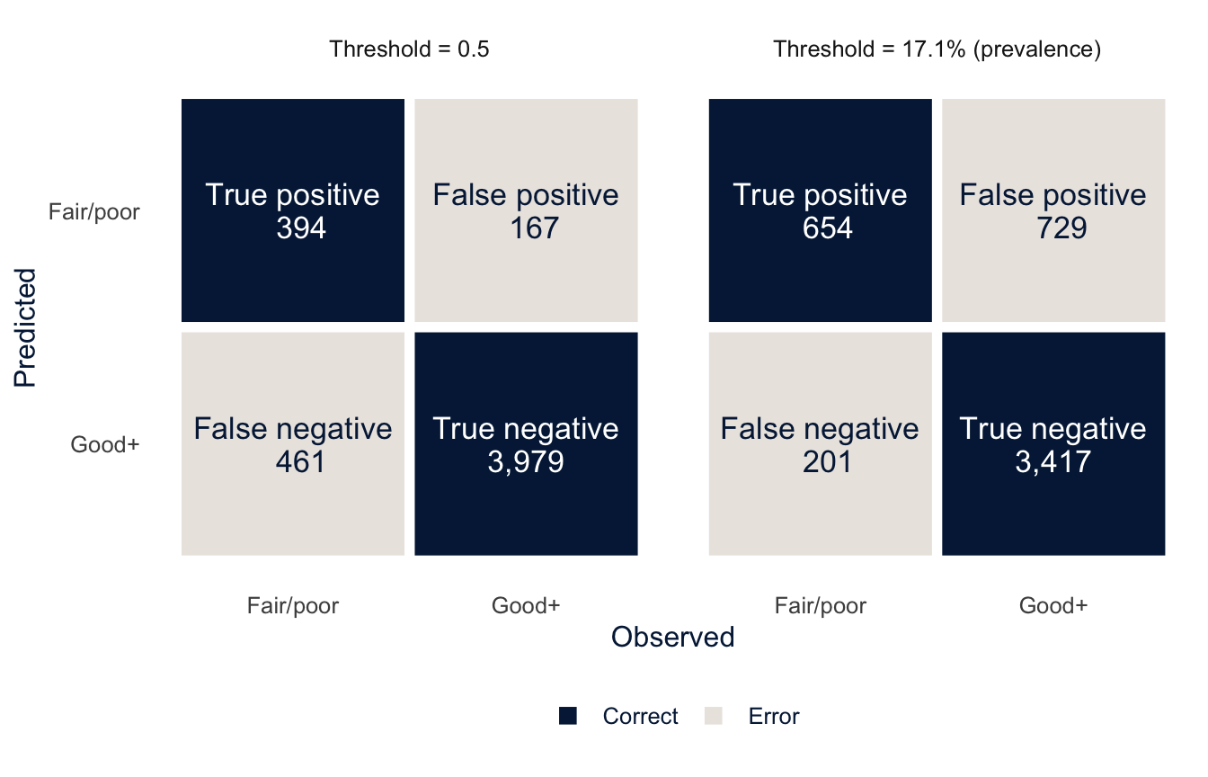

Figure 15.6: Confusion matrices for the boosted tree model on the test set, at two thresholds. The diagonal cells are correct classifications.

NoteCode explanation: drawing a confusion matrix

1. pivot_longer() stacks the two sets of predicted classes into one column, predicted, with rule saying which threshold each row came from. count() then counts the people in each combination of threshold, observed class and predicted class: the cells of the two matrices.
2. case_when() names each cell, and result marks whether it is a correct classification (the diagonal) or an error.
3. geom_tile() draws a rectangle centered on each combination of x and y, which is all a confusion matrix is. The white colour and thick linewidth draw gaps between the tiles.
4. scale_colour_identity() tells ggplot that the text_colour column already holds colors, so it should use them as they are instead of mapping them to a palette. That’s how the labels are white on the dark tiles and dark on the light ones.
5. scale_y_discrete(limits = rev) reverses the order of the rows so that “Fair/poor” is on top, matching the printed conf_mat(). The [[1]] after utsa_cols() drops the name from the color (utsa_cols("midnight") returns a named vector), which scale_fill_manual() would otherwise get confused by.

Read the left panel one cell at a time. The true positives are the 394 people in fair or poor health whom the model classified that way. The true negatives are the 3,979 people in good or better health whom it correctly left alone. The two errors are different kinds of mistakes, and in practice they usually have different costs. The 167 false positives are healthy people the model flags (a wasted outreach call). The 461 false negatives are people in fair or poor health that it misses (someone who needed help and didn’t get it). At a threshold of 0.5, the model misses more people in fair or poor health than it catches. Lowering the threshold to the prevalence, in the right panel, cuts the false negatives to 201, at the price of 729 false positives. Every threshold gives a different confusion matrix, and the choice between them is a choice about which mistake you’d rather make.

Metrics from the confusion matrix

With TP, TN, FP and FN for the four cells and \(N\) for the total, these are the measures you’ll meet most often.

Metric	Formula	Question it answers
Accuracy	\(\frac{TP + TN}{N}\)	What share of everyone is classified correctly?
Sensitivity (recall, true positive rate)	\(\frac{TP}{TP + FN}\)	Of the people in fair or poor health, what share does the model catch?
Specificity (true negative rate)	\(\frac{TN}{TN + FP}\)	Of the people in good health, what share does it correctly leave alone?
Positive predictive value (PPV, precision)	\(\frac{TP}{TP + FP}\)	Of the people the model flags, what share really are in fair or poor health?
Negative predictive value (NPV)	\(\frac{TN}{TN + FN}\)	Of the people it doesn’t flag, what share really are in good health?
Balanced accuracy	\(\frac{\text{sensitivity} + \text{specificity}}{2}\)	What would accuracy be if the two classes were the same size?
F1 score (F measure)	\(\frac{2 \times \text{PPV} \times \text{sensitivity}}{\text{PPV} + \text{sensitivity}}\)	How well does the model do on the positive class alone? (It ignores TN.)
Cohen’s kappa (\(\kappa\))	\(\frac{\text{accuracy} - p_e}{1 - p_e}\)	How much better than chance agreement is the model?

In kappa, \(p_e\) is the accuracy you’d expect if the predictions were made at random, with the same shares of each predicted class as the model gives. Sensitivity and specificity divide by the columns of the confusion matrix (the truth), and PPV and NPV divide by the rows (the predictions). That difference turns out to matter a lot, as we’ll see in a moment.

You can compute any of these by hand from the matrix. At a threshold of 0.5, the sensitivity is 394 / (394 + 461) = 0.461. yardstick has a function for each of them.

class_metrics <- metric_set(accuracy, sensitivity, specificity, ppv, npv,
                            bal_accuracy, f_meas, kap)

cm_metrics <- test_class |>
  pivot_longer(c(pred_05, pred_prev), names_to = "rule", values_to = "predicted") |>
  mutate(threshold = if_else(rule == "pred_05", "0.5", "Prevalence")) |>
  group_by(model, threshold) |>
  class_metrics(truth = badhealth, estimate = predicted)

cm_metrics |>
  select(model, threshold, .metric, .estimate) |>
  pivot_wider(names_from = .metric, values_from = .estimate) |>
  knitr::kable(digits = 3)

model	threshold	accuracy	sensitivity	specificity	ppv	npv	bal_accuracy	f_meas	kap
Boosted trees	0.5	0.874	0.461	0.960	0.702	0.896	0.710	0.556	0.487
Boosted trees	Prevalence	0.814	0.765	0.824	0.473	0.944	0.795	0.584	0.473
Logit	0.5	0.874	0.435	0.964	0.715	0.892	0.700	0.541	0.473
Logit	Prevalence	0.826	0.731	0.846	0.494	0.938	0.788	0.590	0.484

NoteCode explanation: class metrics in yardstick

1. metric_set(), which we used for tuning, bundles several metrics into one function. Here every metric takes predicted classes (estimate = predicted), not probabilities, so I can’t mix in roc_auc or brier_class, which need the probability column.
2. ppv() and npv() are the predictive values, bal_accuracy() is balanced accuracy, f_meas() is the F1 score and kap() is Cohen’s kappa. precision() and recall() also exist; they give the same numbers as ppv() and sensitivity(), under the names used in computer science.
3. Grouping by model and threshold before calling the metric set gives one estimate per metric for each of the four combinations, in long format, and pivot_wider() turns it into one row per combination.

Four things stand out.

1. Accuracy is misleading when the outcome is uncommon. At a threshold of 0.5, the boosted trees classify 87.4% of the test set correctly. That sounds good until you remember that only 17.1% of people are in fair or poor health, so a “model” that says everyone is in good health would be right 82.9% of the time. This benchmark is called the no-information rate, and you should always compare accuracy with it.
2. The threshold trades sensitivity for specificity. Moving from 0.5 to the prevalence raises the boosted trees’ sensitivity from 46.1% to 76.5% and lowers specificity from 96.0% to 82.4%. Accuracy falls, even though the model now catches far more of the people we care about. Balanced accuracy, which counts the two classes equally, rises. The threshold is a decision, not an estimate, and the metric you judge it by should match what the decision is for.
3. Measures that ignore the true negatives tell a different story. The F1 score and kappa change much less with the threshold than sensitivity and specificity do, because they balance gains in one cell against losses in another. They’re useful single numbers for comparing models, but they hide the tradeoff, so report the confusion matrix alongside them.
4. The two models are almost interchangeable, again. Whatever threshold you choose, the logit and the boosted trees make about the same number of each kind of mistake.

Predictive values depend on prevalence

At the prevalence threshold, only 47.3% of the people the boosted trees flag are actually in fair or poor health (the PPV). That isn’t a flaw peculiar to this model. Sensitivity and specificity describe how the model treats people given their true status, so they don’t depend on how common the outcome is. PPV and NPV describe who ends up in each predicted group, and that depends on how many people with and without the outcome there are to begin with. By Bayes’ theorem,

\[ \text{PPV} = \frac{\text{sensitivity} \times p}{\text{sensitivity} \times p + (1 - \text{specificity}) \times (1 - p)}, \]

where \(p\) is the prevalence. The figure holds the model’s sensitivity and specificity fixed and varies \(p\).

sens <- get_cm("Boosted trees", "Prevalence", "sensitivity")
spec <- get_cm("Boosted trees", "Prevalence", "specificity")

tibble(prevalence = seq(0.01, 0.6, by = 0.01)) |>
  mutate(PPV = sens * prevalence / (sens * prevalence + (1 - spec) * (1 - prevalence)),
         NPV = spec * (1 - prevalence) / (spec * (1 - prevalence) + (1 - sens) * prevalence)) |>
  pivot_longer(c(PPV, NPV), names_to = "metric", values_to = "value") |>
  ggplot(aes(x = prevalence, y = value, colour = metric, linetype = metric)) +
  geom_vline(xintercept = prev, colour = utsa_cols("midnight"), linetype = "dotted") +
  geom_line(linewidth = 1.1) +
  scale_colour_utsa(palette = "primary") +
  scale_x_continuous(labels = scales::label_percent()) +
  scale_y_continuous(labels = scales::label_percent(), limits = c(0, 1)) +
  labs(x = "Prevalence of fair or poor health", y = "Predictive value",
       colour = NULL, linetype = NULL)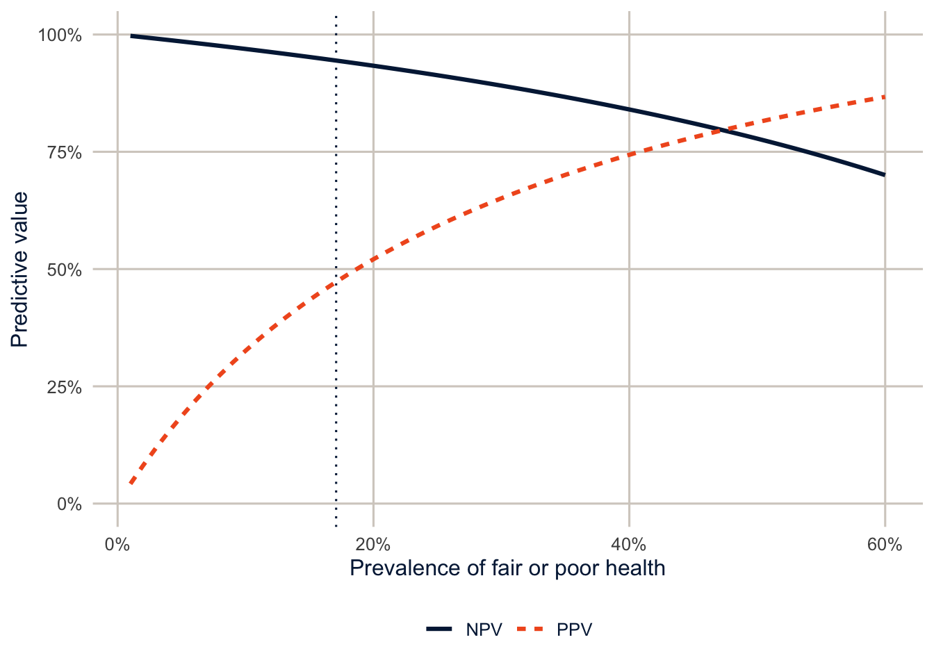

Figure 15.7: Positive and negative predictive values of the boosted tree model (prevalence threshold) at different prevalences of fair or poor health, holding its sensitivity and specificity fixed. The vertical line marks the prevalence in the training data.

The same model, with the same sensitivity and specificity, would have a PPV of about 19% in a population where 5% are in fair or poor health, and about 65% in one where 30% are. This is the familiar problem of screening for rare conditions, and it matters for demographers because prevalence differs across groups. In the test set, fair or poor health is much more common among Hispanic adults than NH White adults, so even a model with identical sensitivity and specificity in both groups would have a higher PPV for Hispanic adults and a lower NPV. Keep this in mind for the section on fairness and for exercise 3, which computes these metrics by race and ethnicity.

Which metric should you report? It depends on what the predictions are for. A screening program that wants to miss as few people as possible cares most about sensitivity. A program with a fixed number of slots, which can only follow up with the people it flags, cares about PPV, because every false positive takes a slot. When in doubt, report the confusion matrix and let readers compute what they need.

bind_rows(collect_predictions(final_logit) |> mutate(model = "Logit"),
          collect_predictions(final_xgb) |> mutate(model = "Boosted trees")) |>
  group_by(model) |>
  roc_curve(badhealth, `.pred_Fair/poor`) |>
  ggplot(aes(x = 1 - specificity, y = sensitivity, colour = model, linetype = model)) +
  geom_abline(colour = utsa_cols("smoke")) +
  geom_path(linewidth = 1.1) +
  coord_equal() +
  scale_colour_utsa(palette = "primary") +
  labs(x = "False positive rate (1 - specificity)", y = "True positive rate (sensitivity)",
       colour = NULL, linetype = NULL)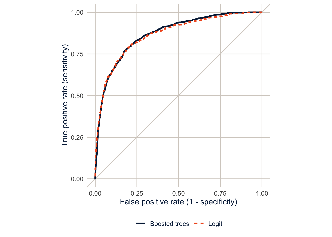

Figure 15.8: ROC curves for the logit and boosted tree models on the test set.

The ROC curve ties the threshold back to the AUC. Each point on it is one confusion matrix: the sensitivity and the false positive rate (1 − specificity) at one threshold. The curve traces those pairs as the threshold moves from 1 (bottom left, nobody flagged) down to 0 (top right, everybody flagged), and the AUC is the area under it, a summary over every possible threshold. The two ROC curves lie almost on top of each other.

What does the model use?

A random forest or boosted model has no coefficients to read, but you can ask how much each predictor contributes. Variable importance for a random forest adds up how much each predictor’s splits improve the fit across all the trees.

final_rf <- wf_rf |>
  finalize_workflow(select_best(res_rf, metric = "roc_auc")) |>
  fit(train)

extract_fit_engine(final_rf)$variable.importance |>
  enframe(name = "variable", value = "importance") |>
  slice_max(importance, n = 12) |>
  ggplot(aes(x = importance, y = fct_reorder(variable, importance))) +
  geom_col(fill = utsa_cols("midnight")) +
  labs(x = "Importance", y = NULL)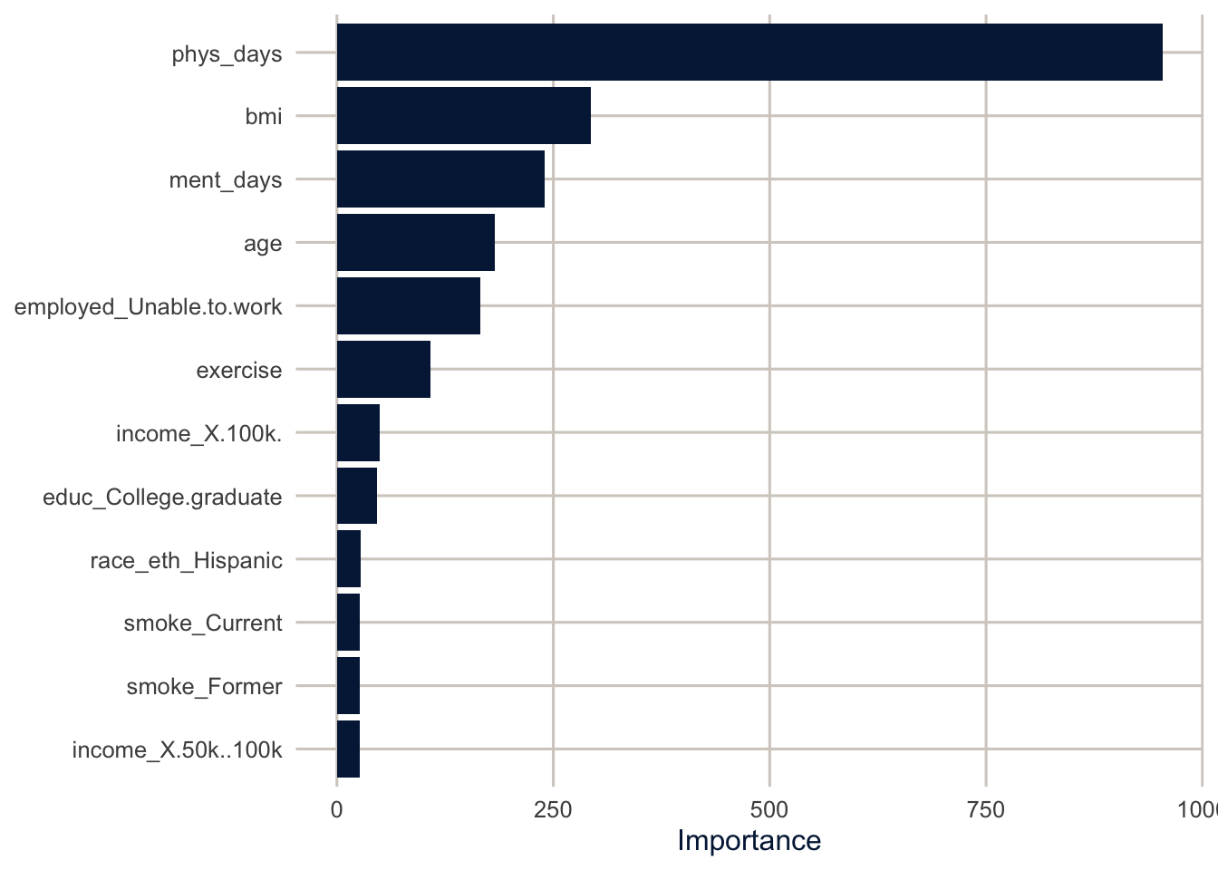

Figure 15.9: Variable importance from the random forest (total decrease in node impurity), fit to the training data.

The number of poor physical health days dominates, followed by BMI, poor mental health days, the employment category “unable to work,” and age. None of that is surprising, and that’s worth noticing. Machine learning mostly rediscovered what a demographer would have put in the model in the first place. Importance measures model reliance: what this model uses to make its predictions. It isn’t a causal effect, or even an association you could interpret like a coefficient. Physical health days and inability to work are partly consequences of poor health, which is fine for prediction and useless for explanation. And when two predictors carry similar information, the model may lean on one and ignore the other, so a low importance doesn’t mean a variable is unrelated to the outcome.

Calibration

A good ranking isn’t enough if you’re going to use the predicted probabilities themselves, say, to estimate how many people in a county are in fair or poor health. A model is calibrated if, among people with a predicted probability of 20%, about 20% have the outcome. Check by grouping people by their predicted probability and comparing the average prediction with the observed share in each group.

bind_rows(collect_predictions(final_logit) |> mutate(model = "Logit"),
          collect_predictions(final_xgb) |> mutate(model = "Boosted trees")) |>
  group_by(model, bin = ntile(`.pred_Fair/poor`, 10)) |>
  summarise(predicted = mean(`.pred_Fair/poor`),
            observed = mean(badhealth == "Fair/poor"), .groups = "drop") |>
  ggplot(aes(x = predicted, y = observed, colour = model, shape = model)) +
  geom_abline(colour = utsa_cols("smoke")) +
  geom_line() +
  geom_point(size = 2.5) +
  coord_equal() +
  scale_colour_utsa(palette = "primary") +
  scale_x_continuous(labels = scales::label_percent()) +
  scale_y_continuous(labels = scales::label_percent()) +
  labs(x = "Mean predicted probability (deciles)", y = "Observed share in fair/poor health",
       colour = NULL, shape = NULL)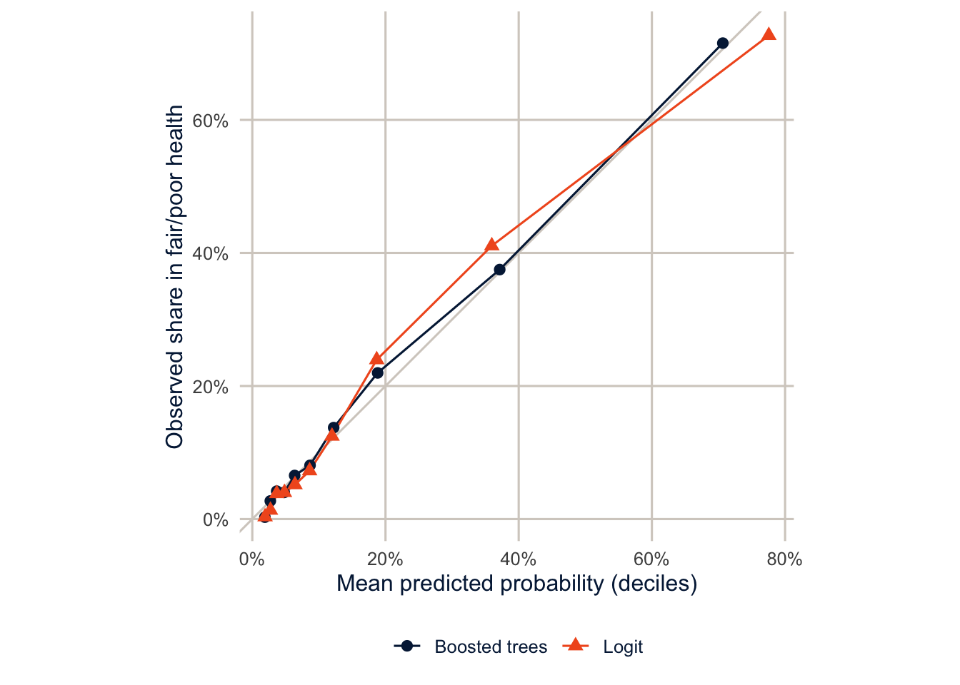

Figure 15.10: Calibration of the logit and boosted tree models on the test set. Points on the diagonal are perfectly calibrated.

NoteCode explanation: a calibration plot by hand

ntile(x, 10) splits the predictions into ten groups of equal size, from lowest to highest. Within each group, I compare the mean predicted probability with the share who actually reported fair or poor health. The probably package has functions that draw these plots for you (cal_plot_breaks()), but they’re only a few lines of dplyr, and doing it yourself makes clear what the plot shows.

Both models are reasonably well calibrated on the test data, with points near the diagonal. That’s typical of a logit model fit to a large sample, but it isn’t guaranteed for any model: a logit model can be poorly calibrated on new data if it’s misspecified, or if the new data come from a different population. Random forests and boosted trees are more often miscalibrated, especially with small learning rates or few trees. Whatever the model, check calibration on data it wasn’t fit to before using its probabilities as probabilities.

TipReading the result: a right and a wrong interpretation

Right: “On the test set, the boosted tree model ranks people in fair or poor health above people in good health with an AUC of 0.87, and its predicted probabilities are close to the observed shares across deciles of risk.”

Wrong: “The model has an AUC of 0.87, so its predicted probabilities are accurate.” The AUC only measures ranking. A model can rank people well and still systematically over- or underestimate everyone’s risk; that’s what the calibration plot is for.

Fairness

Does the model work equally well for everyone?

A model that predicts well on average can predict badly for some groups. That matters if predictions are used to make decisions about people. Obermeyer et al. (2019) studied an algorithm used by U.S. health systems to decide who got extra care management. It predicted health care costs as a stand-in for health care needs, and because less money is spent on Black patients with the same level of illness, it systematically underestimated how sick Black patients were. Fixing the target variable roughly tripled the share of Black patients flagged for extra care.

Here is our model’s performance by race and ethnicity, in the test set.

preds <- collect_predictions(final_xgb) |>
  bind_cols(select(test, race_eth))

auc_group <- preds |>
  group_by(race_eth) |>
  roc_auc(badhealth, `.pred_Fair/poor`) |>
  select(race_eth, auc = .estimate)

calib_group <- preds |>
  group_by(race_eth) |>
  summarise(n = n(),
            observed = mean(badhealth == "Fair/poor"),
            predicted = mean(`.pred_Fair/poor`))

left_join(calib_group, auc_group, by = "race_eth") |>
  mutate(difference = predicted - observed) |>
  knitr::kable(digits = 3)

race_eth	n	observed	predicted	auc	difference
NH White	3582	0.153	0.158	0.881	0.005
NH Black	465	0.185	0.196	0.806	0.011
NH Other	251	0.155	0.144	0.862	-0.011
NH Multiracial	97	0.227	0.182	0.789	-0.044
Hispanic	606	0.264	0.213	0.855	-0.051

NoteCode explanation: binding predictions to the test data

collect_predictions() returns the predictions for the test set in the same row order as the test data, so bind_cols() can attach the race and ethnicity column. Grouping by it and calling roc_auc() computes the AUC within each group.

The model ranks people best among NH White adults (AUC 0.88) and less well for Hispanic adults (0.85) and NH Black adults (0.81). Look at the calibration columns too: if the predicted share is below the observed share for a group, the model underestimates how many people in that group are in poor health, and anyone using it to allocate resources by predicted need would shortchange them. That’s what happens for Hispanic adults: the model predicts that 21.3% are in fair or poor health, and 26.4% actually are. These test-set groups are small (some have only a few hundred people), so these differences are noisy, and you’d want to confirm them with more data or cross-validation before acting on them. A subgroup AUC or calibration difference should come with a measure of its uncertainty (bootstrapping the test set is the simplest way), just like any other estimate. But this is exactly the check to do, and most published prediction models never report it.

There’s a harder problem underneath, too. “Fair” has several reasonable definitions: equal calibration in every group, equal sensitivity, equal false positive rates, equal PPV. When the outcome is more common in some groups than others, as it is here, a model generally can’t satisfy all of them at once. The PPV figure above showed one reason: with the same sensitivity and specificity, the group with the higher prevalence gets a higher PPV. So choosing a fairness criterion is a decision about which kind of unequal treatment matters most for the use at hand, not a technical setting.

Why would a model work less well for some groups? Because they’re a minority of the training data, so the model learns less about them. Because the predictors mean different things in different groups (an income of $50,000 goes further in some places than others, and self-rated health questions may be answered differently across languages and cultures). And because the outcome itself can be measured differently, as in the Obermeyer study.

Limits of prediction for policy

Three cautions before you use a predictive model to make decisions about people.

1. A prediction is not a reason. A model that predicts poor health from being unable to work doesn’t tell you that finding people jobs will improve their health. If the decision is about intervening, you’re back to the causal questions of week 14.
2. Check performance by group, and check calibration, not just overall accuracy. Report both. Decide in advance what level of difference between groups would be unacceptable.
3. Think about what the outcome measures. A model is only as good as its target. If the outcome is a proxy (costs for need, arrests for crime, test scores for learning), the model will reproduce whatever biases the proxy has.

TipSurvey weights in tidymodels

I ignored the survey weights here, which is common in prediction, where the goal is to predict well for the sample at hand. If the model is meant to predict well for the population, tidymodels supports case weights: wrap the weight with importance_weights() in the data, and add add_case_weights() to the workflow. Weighted metrics are also available in yardstick. See Kuhn and Silge (2022) for the details.

Summary

Prediction is a different goal from explanation: we judge models on data they haven’t seen, using a held-out test set and cross-validation, and flexibility is a tool rather than a danger. Trees split the data into groups with a series of yes/no questions; random forests average many trees grown on bootstrap samples, and boosted trees add up many shallow trees fit to each other’s errors. In survey data with a few categorical predictors, a well-specified logit model often predicts as well as either, so always fit a baseline. Check calibration as well as discrimination, and check both for each group the model will be used on. A prediction is not a causal effect, and a model that predicts well on average can still fail the people who most need it to work. James et al. (2021) is a free, readable introduction to the methods, and Kuhn and Silge (2022) covers tidymodels.

Homework 15

Due: May 6, before class.

Which version to do. If you’re in DEM 7283, do the version with your own survey data. If you’re in DEM 5283, do either version, and say at the top of your homework which one you did. If your survey can’t support this week’s method, do the version with my data and say so.

Purpose. Build and evaluate prediction models for a stated use, and judge them by what the use needs.

A satisfactory answer ties each evaluation to a prediction use; keeps discrimination, calibration and decision consequences separate; compares flexible models with a simple baseline; and treats subgroup differences as estimates with uncertainty, not as settled facts.

With your own survey data

Use the full survey design for every estimate unless a step says otherwise, and report each estimate with a standard error or confidence interval.

1. Choose a binary outcome to predict, and say who would use the predictions and what they would do with them.
2. Split your data into training and test sets, stratified on the outcome, and write a recipe to prepare your predictors.
3. Fit three models on the training data:
   • a logistic regression;
   • a random forest; and
   • a boosted tree model.
4. Tune the random forest and boosted tree with 5- or 10-fold cross-validation, and compare all three models by cross-validated ROC AUC. Which do you choose?
5. Evaluate your chosen model on the test data:
   1. Report the ROC AUC and show the ROC curve.
   2. Show a calibration plot. Are the predicted probabilities trustworthy?
   3. Choose a classification threshold for the use you described in step 1, justify it, and report the confusion matrix, sensitivity, specificity and positive predictive value.
6. Show the variable importance for your chosen model. Explain why importance isn’t the same as a causal effect.
7. Compare the model’s performance across two or more groups (for example, by race and ethnicity or sex). Does it perform equally well for everyone? What would the consequences be if it didn’t?
8. These models don’t use the survey design. What population does your model’s performance describe, and how would you adjust your evaluation to describe the population the survey represents?

With my data

What is provided. The BRFSS sample brfss, the split, training and test data and folds, the recipe and model specifications, and the tuned models from this chapter.

1. Figure 15.2 chose a tree depth using a single fold. Do it properly: tune tree_depth from 1 to 12 with tune_grid() and all five folds (set cost_complexity = -1, and use grid = tibble(tree_depth = 1:12)). Which depth gives the best cross-validated AUC? Draw that tree with rpart.plot() and describe its first three questions in words. How does its cross-validated AUC compare with the random forest’s?

# YOUR CODE HERE

One solution for exercise 1

wf_tree <- workflow(badhealth ~ .,
                    decision_tree(tree_depth = tune(), cost_complexity = -1) |>
                      set_mode("classification"))
res_tree <- tune_grid(wf_tree, folds, grid = tibble(tree_depth = 1:12), metrics = metrics)
show_best(res_tree, metric = "roc_auc", n = 3)

fit_tree <- wf_tree |>
  finalize_workflow(select_best(res_tree, metric = "roc_auc")) |>
  fit(train)
rpart.plot(extract_fit_engine(fit_tree), roundint = FALSE)

2. Remove the two variables that are closest to being measures of the outcome itself, phys_days and ment_days, and refit the logit and random forest models with cross-validation. How much does performance drop? Which predictors become most important?

# YOUR CODE HERE

3. Using the logit model from the test set, compute the sensitivity and specificity by race and ethnicity at a threshold equal to the overall prevalence of fair or poor health (the week 4 decision rule). Would a program that used this rule to offer services treat the groups equally?

# YOUR CODE HERE

4. Refit the boosted tree model with trees = 1000 and compare its cross-validated AUC and Brier score with the 300-tree model. Is the extra computing time worth it?

# YOUR CODE HERE

5. Describe an intended use for a model predicting fair or poor health, different from the one in this chapter: who would be predicted, when, and what decision it would support. List which of this chapter’s predictors would be available at that time. Then compare a simple model (the logit) and a flexible one (random forest or boosted trees) on both discrimination and calibration for that set of predictors. Explain one consequence of a false positive and one of a false negative for your use, and compare the model’s performance for two racial and ethnic groups, saying how much the comparison could be due to chance.

Additional resources

• Tidy Modeling with R (Kuhn and Silge 2022), free online, is the full guide to the tidymodels framework used in this chapter.
• An Introduction to Statistical Learning (James et al. 2021), free online, explains trees, random forests and boosting with as little math as the subject allows.
• Molina and Garip (2019), “Machine Learning for Sociology,” Annual Review of Sociology, on where prediction helps social science and where it doesn’t.
• Barocas, Hardt and Narayanan, Fairness and Machine Learning, free online, for a much longer look at the questions at the end of this chapter.

Breiman, Leo. 2001. “Random Forests.” Machine Learning 45 (1): 5–32.

Chen, Tianqi, and Carlos Guestrin. 2016. “XGBoost: A Scalable Tree Boosting System.” Proceedings of the 22nd ACM SIGKDD International Conference on Knowledge Discovery and Data Mining, 785–94.

James, Gareth, Daniela Witten, Trevor Hastie, and Robert Tibshirani. 2021. An Introduction to Statistical Learning with Applications in R. 2nd ed. Springer.

Kuhn, Max, and Julia Silge. 2022. Tidy Modeling with R: A Framework for Modeling in the Tidyverse. O’Reilly Media. https://www.tmwr.org.

Molina, Mario, and Filiz Garip. 2019. “Machine Learning for Sociology.” Annual Review of Sociology 45: 27–45.

Obermeyer, Ziad, Brian Powers, Christine Vogeli, and Sendhil Mullainathan. 2019. “Dissecting Racial Bias in an Algorithm Used to Manage the Health of Populations.” Science 366 (6464): 447–53.